付録
The Use of Mathematics in Principles of Economics経済学原理における数学の利用
(This appendix should be consulted after first reading Welcome to Economics!) Economics is not math. There is no important concept in this course that cannot be explained without mathematics. That said, math is a tool that can be used to illustrate economic concepts. Remember the saying a picture is worth a thousand words? Instead of a picture, think of a graph. It is the same thing. Economists use models as the primary tool to derive insights about economic issues and problems. Math is one way of working with (or manipulating) economic models.
英語のヒント
(この付録は、まず「経済学へようこそ」を読んでから参照しよう。)経済学は数学ではない。この講義の重要な概念は、どれも数学なしで説明できる。それでも、数学は経済概念を示すための道具として使える。「百聞は一見にしかず」という言葉を思い出そう。絵の代わりにグラフを考えても同じだ。経済学者は、経済の課題や問題を理解する主要な道具としてモデルを使う。数学は、経済モデルを扱い、操作する方法の一つである。
There are other ways of representing models, such as text or narrative. But why would you use your fist to bang a nail, if you had a hammer? Math has certain advantages over text. It disciplines your thinking by making you specify exactly what you mean. You can get away with fuzzy thinking in your head, but you cannot when you reduce a model to algebraic equations. At the same time, math also has disadvantages. Mathematical models are necessarily based on simplifying assumptions, so they are not likely to be perfectly realistic. Mathematical models also lack the nuances which can be found in narrative models. The point is that math is one tool, but it is not the only tool or even always the best tool economists can use. So what math will you need for this book? The answer is: little more than high school algebra and graphs. You will need to know:
英語のヒント
モデルは文章や物語などでも表せる。しかし、金槌があるのに、なぜ拳で釘を打つだろうか。数学には文章に勝る点がある。何を意味するのか正確に指定させることで、思考を整える。頭の中では曖昧に考えても済むが、モデルを代数方程式にするとそうはいかない。同時に欠点もある。数学モデルは必ず単純化の仮定に基づくので、完全に現実的とは考えにくい。物語型のモデルにある細やかな意味合いも欠ける。数学は一つの道具であり、唯一でも、常に最善でもない。この本に必要な数学は何か。答えは、高校の代数とグラフを少し知っている程度だ。次のことを理解しておく必要がある。
- What a function is
英語のヒント
関数とは何か - How to interpret the equation of a line (i.e., slope and intercept)
英語のヒント
直線の方程式、すなわち傾きと切片をどう読み取るか - How to manipulate a line (i.e., changing the slope or the intercept)
英語のヒント
傾きや切片を変えることで、直線をどう動かすか - How to compute and interpret a growth rate (i.e., percentage change)
英語のヒント
成長率、すなわち変化率(%)をどう計算して解釈するか - How to read and manipulate a graph
英語のヒント
グラフをどう読み、操作するか
In this text, we will use the easiest math possible, and we will introduce it in this appendix. So if you find some math in the book that you cannot follow, come back to this appendix to review. Like most things, math has diminishing returns. A little math ability goes a long way; the more advanced math you bring in, the less additional knowledge that will get you. That said, if you are going to major in economics, you should consider learning a little calculus. It will be worth your while in terms of helping you learn advanced economics more quickly.
英語のヒント
本書ではできるだけ易しい数学を使い、この付録で紹介する。理解できない数学が本文に出てきたら、ここへ戻って復習しよう。ほかの多くのものと同じく、数学にも収穫逓減がある。少しの数学で大いに役立つが、高度な数学を追加するほど、得られる知識の上積みは小さくなる。とはいえ、経済学を専攻するなら、微積分を少し学ぶことを考えよう。より高度な経済学を速く学ぶ助けとなり、その価値はある。
Algebraic Models代数によるモデル
Often economic models (or parts of models) are expressed in terms of mathematical functions. What is a function? A function describes a relationship. Sometimes the relationship is a definition. For example (using words), your professor is Adam Smith. This could be expressed as Professor = Adam Smith. Or Friends = Bob + Shawn + Margaret.
英語のヒント
経済モデルやその一部は、数学的な関数で表されることが多い。関数とは何か。関数は関係を記述する。定義を表すこともある。例えば、言葉では「あなたの教授はアダム・スミスである」という関係を、「教授=アダム・スミス」と書ける。「友人=ボブ+ショーン+マーガレット」でもよい。
Often in economics, functions describe cause and effect. The variable on the left-hand side is what is being explained (“the effect”). On the right-hand side is what is doing the explaining (“the causes”). For example, suppose your GPA was determined as follows:
英語のヒント
経済学では、関数が因果関係を示すことが多い。左辺の変数は説明されるもの、つまり「結果」であり、右辺は説明するもの、つまり「原因」だ。例えば、成績平均値GPAが次のように決まるとしよう。
This equation states that your GPA depends on three things: your combined SAT score, your class attendance, and the number of hours you spend studying. It also says that study time is twice as important (0.50) as either combined_SAT score (0.25) or class_attendance (0.25). If this relationship is true, how could you raise your GPA? By not skipping class and studying more. Note that you cannot do anything about your SAT score, since if you are in college, you have (presumably) already taken the SATs.
英語のヒント
この式では、GPAはSAT総合点、授業への出席、勉強時間の三つによって決まる。また勉強時間の重要度0.50は、SAT総合点0.25や出席0.25の2倍だとしている。この関係が正しければ、どうすればGPAを上げられるか。授業を休まず、もっと勉強すればよい。大学にいるなら、おそらくSATはすでに受験済みなので、その点数は変えられないことに注意しよう。
Of course, economic models express relationships using economic variables, like Budget = money_spent_on_econ_books + money_spent_on_music, assuming that the only things you buy are economics books and music.
英語のヒント
もちろん経済モデルは、経済変数を使って関係を表す。例えば、買う物が経済学の本と音楽だけだと仮定すれば、「予算=経済学の本に使うお金+音楽に使うお金」となる。
Most of the relationships we use in this course are expressed as linear equations of the form:
英語のヒント
この講義で使う関係の多くは、次の形の一次方程式で表される。
Expressing Equations Graphically
英語のヒント
方程式をグラフで表す
Graphs are useful for two purposes. The first is to express equations visually, and the second is to display statistics or data. This section will discuss expressing equations visually.
英語のヒント
グラフには二つの用途がある。一つは方程式を視覚的に表すこと、もう一つは統計やデータを示すことだ。この節では方程式の視覚的な表現を扱う。
To a mathematician or an economist, a variable is the name given to a quantity that may assume a range of values. In the equation of a line presented above, x and y are the variables, with x on the horizontal axis and y on the vertical axis, and b and m representing factors that determine the shape of the line. To see how this equation works, consider a numerical example:
英語のヒント
数学者や経済学者にとって変数とは、さまざまな値を取り得る数量に付けた名前である。上の直線の方程式ではxとyが変数で、横軸にx、縦軸にyを取る。bとmは直線の形を決める要因だ。式の働きを見るため、数値例を考えよう。
In this equation for a specific line, the b term has been set equal to 9 and the m term has been set equal to 3. Table A.1 shows the values of x and y for this given equation. Figure A.1 shows this equation, and these values, in a graph. To construct the table, just plug in a series of different values for x, and then calculate what value of y results. In the figure, these points are plotted and a line is drawn through them.
英語のヒント
x |
y |
|---|---|
0 |
9 |
1 |
12 |
2 |
15 |
3 |
18 |
4 |
21 |
5 |
24 |
6 |
27 |
Slope and the Algebra of Straight Lines傾きと直線の代数
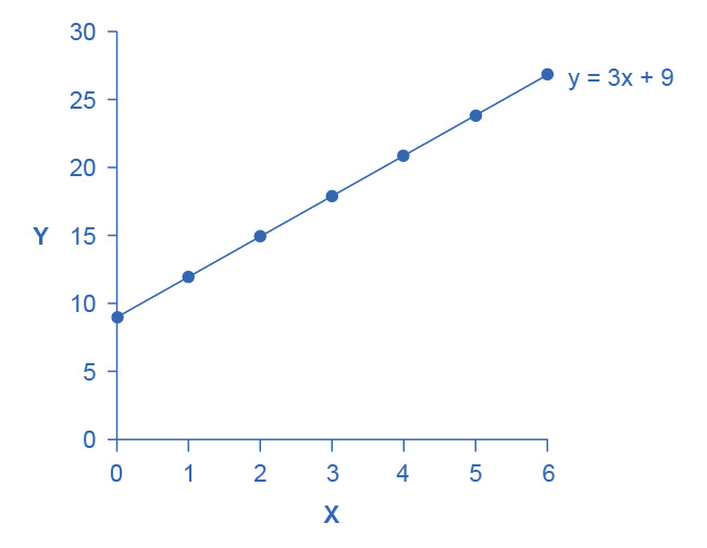
Figure A.1図 A.1
This line graph has x on the horizontal axis and y on the vertical axis. The y-intercept—that is, the point where the line intersects the y-axis—is 9. The slope of the line is 3; that is, there is a rise of 3 on the vertical axis for every increase of 1 on the horizontal axis. The slope is the same all along a straight line.
英語のヒント
横軸にx、縦軸にyを取る。y切片、すなわち直線がy軸と交わる値は9だ。傾きは3で、横軸の値が1増えるたび、縦軸の値が3増える。直線の傾きはどこでも同じである。
This example illustrates how the b and m terms in an equation for a straight line determine the shape of the line. The b term is called the y-intercept. The reason for this name is that, if x = 0, then the b term will reveal where the line intercepts, or crosses, the y-axis. In this example, the line hits the vertical axis at 9. The m term in the equation for the line is the slope. Remember that slope is defined as rise over run; more specifically, the slope of a line from one point to another is the change in the vertical axis divided by the change in the horizontal axis. In this example, each time the x term increases by one (the run), the y term rises by three. Thus, the slope of this line is three. Specifying a y-intercept and a slope—that is, specifying b and m in the equation for a line—will identify a specific line. Although it is rare for real-world data points to arrange themselves as an exact straight line, it often turns out that a straight line can offer a reasonable approximation of actual data.
英語のヒント
この例は、直線の式のbとmが形をどう決めるかを示す。bはy切片と呼ばれる。x=0のとき、bが直線とy軸の交わる位置を示すためだ。この例では縦軸の9で交わる。mは傾きだ。傾きは「縦の変化÷横の変化」と定義する。つまり、一つの点から別の点への縦軸の変化を、横軸の変化で割ったものだ。この例ではxが1増えるたびにyが3増えるので、傾きは3になる。y切片と傾き、すなわちbとmを指定すれば、特定の直線が決まる。現実のデータが正確な直線上に並ぶことはまれだが、直線で妥当に近似できることは多い。
Interpreting the Slope
英語のヒント
傾きの解釈
The concept of slope is very useful in economics, because it measures the relationship between two variables. A positive slope means that two variables are positively related; that is, when x increases, so does y, or when x decreases, y decreases also. Graphically, a positive slope means that as a line on the line graph moves from left to right, the line rises. The length-weight relationship, shown in Figure A.3 later in this Appendix, has a positive slope. We will learn in other chapters that price and quantity supplied have a positive relationship; that is, firms will supply more when the price is higher.
英語のヒント
傾きは二つの変数の関係を測るので、経済学で非常に役立つ。正の傾きは正の関係を意味する。xが増えればyも増え、xが減ればyも減る。グラフでは左から右へ進むと線が上がる。この付録の後の図A.3に示す体長と体重の関係は、正の傾きを持つ。ほかの章では、価格と供給量に正の関係があることを学ぶ。価格が高いほど、企業は多く供給する。
A negative slope means that two variables are negatively related; that is, when x increases, y decreases, or when x decreases, y increases. Graphically, a negative slope means that, as the line on the line graph moves from left to right, the line falls. The altitude-air density relationship, shown in Figure A.4 later in this appendix, has a negative slope. We will learn that price and quantity demanded have a negative relationship; that is, consumers will purchase less when the price is higher.
英語のヒント
負の傾きは、二つの変数が負の関係にあることを意味する。xが増えるとyが減り、xが減るとyが増える。グラフでは、左から右へ進むと線が下がる。後の図A.4の高度と空気密度の関係は、負の傾きを持つ。価格と需要量にも負の関係があり、価格が高いほど消費者の購入量が減ることを学ぶ。
A slope of zero means that there is no relationship between x and y. Graphically, the line is flat; that is, zero rise over the run. Figure A.5 of the unemployment rate, shown later in this appendix, illustrates a common pattern of many line graphs: some segments where the slope is positive, other segments where the slope is negative, and still other segments where the slope is close to zero.
英語のヒント
傾きがゼロなら、xとyに関係がないことを意味する。グラフでは線が平らで、横に進んでも縦の変化がゼロだ。後の図A.5の失業率は、多くの折れ線グラフに共通する形を示す。正の傾きの区間、負の区間、ほぼゼロの区間がある。
The slope of a straight line between two points can be calculated in numerical terms. To calculate slope, begin by designating one point as the “starting point” and the other point as the “end point” and then calculating the rise over run between these two points. As an example, consider the slope of the air density graph between the points representing an altitude of 4,000 meters and an altitude of 6,000 meters:
英語のヒント
2点間の直線の傾きは、数値で計算できる。一方を「始点」、他方を「終点」とし、2点間の縦の変化を横の変化で割る。空気密度のグラフで、高度4,000メートルと6,000メートルの点の間の傾きを考えよう。
Rise: Change in variable on vertical axis (end point minus original point)
英語のヒント
縦の変化:縦軸の変数の変化(終点−始点)
Run: Change in variable on horizontal axis (end point minus original point)
英語のヒント
横の変化:横軸の変数の変化(終点−始点)
Thus, the slope of a straight line between these two points would be that from the altitude of 4,000 meters up to 6,000 meters, the density of the air decreases by approximately 0.1 kilograms/cubic meter for each of the next 1,000 meters.
英語のヒント
この2点間の直線の傾きは、高度4,000〜6,000メートルでは1,000メートル上がるごとに空気密度が約0.1キログラム/立方メートル減ることを意味する。
Suppose the slope of a line were to increase. Graphically, that means it would get steeper. Suppose the slope of a line were to decrease. Then it would get flatter. These conditions are true whether or not the slope was positive or negative to begin with. A higher positive slope means a steeper upward tilt to the line, while a smaller positive slope means a flatter upward tilt to the line. A negative slope that is larger in absolute value (that is, more negative) means a steeper downward tilt to the line. A slope of zero is a horizontal flat line. A vertical line has an infinite slope.
英語のヒント
直線の傾きが大きくなると、グラフではより急になる。傾きが小さくなると、より平らになる。これは、元の傾きが正でも負でも当てはまる。正の傾きが大きいほど上向きの傾斜は急で、小さいほど緩い。負の傾きの絶対値が大きい、つまりより負なら、下向きの傾斜は急になる。傾きゼロは水平な直線で、垂直な直線の傾きは無限大である。
Suppose a line has a larger intercept. Graphically, that means it would shift out (or up) from the old origin, parallel to the old line. If a line has a smaller intercept, it would shift in (or down), parallel to the old line.
英語のヒント
直線の切片が大きくなると、元の直線に平行に、元の原点から外側、つまり上へ移動する。切片が小さくなると、平行に内側、つまり下へ移動する。
Solving Models with Algebra
英語のヒント
代数でモデルを解く
Economists often use models to answer a specific question, like: What will the unemployment rate be if the economy grows at 3% per year? Answering specific questions requires solving the “system” of equations that represent the model.
英語のヒント
経済学者はモデルを使って、例えば「経済が年3%成長すると失業率はいくらになるか」という具体的な問いに答える。答えるには、モデルを表す連立方程式を解く必要がある。
Suppose the demand for personal pizzas is given by the following equation:
英語のヒント
1人用ピザの需要が、次の式で与えられるとする。
where Qd is the amount of personal pizzas consumers want to buy (i.e., quantity demanded), and P is the price of pizzas. Suppose the supply of personal pizzas is:
英語のヒント
Qdは消費者が買いたい1人用ピザの量、すなわち需要量、Pはピザの価格である。供給は次のとおりだとする。
where Qs is the amount of pizza producers will supply (i.e., quantity supplied).
英語のヒント
Qsは生産者が供給するピザの量、すなわち供給量である。
Finally, suppose that the personal pizza market operates where supply equals demand, or
英語のヒント
最後に、1人用ピザの市場では、需要と供給が一致する、つまり次の関係が成り立つとする。
We now have a system of three equations and three unknowns (Qd, Qs, and P), which we can solve with algebra:
英語のヒント
これで3本の式と3個の未知数Qd、Qs、Pからなる連立方程式ができた。代数で解ける。
Since Qd = Qs, we can set the demand and supply equation equal to each other:
英語のヒント
Qd=Qsなので、需要と供給の式を等しいと置く。
Subtracting 2 from both sides and adding 2P to both sides yields:
英語のヒント
両辺から2を引き、両辺に2Pを足すと、次のようになる。
In other words, the price of each personal pizza will be $2. How much will consumers buy?
英語のヒント
つまり、1人用ピザ1枚の価格は2ドルになる。消費者は何枚買うだろうか。
Taking the price of $2, and plugging it into the demand equation, we get:
英語のヒント
価格2ドルを需要の式に代入すると、
So if the price is $2 each, consumers will purchase 12. How much will producers supply? Taking the price of $2, and plugging it into the supply equation, we get:
英語のヒント
1枚2ドルなら、消費者は12枚買う。生産者は何枚供給するか。価格2ドルを供給の式に代入すると、
So if the price is $2 each, producers will supply 12 personal pizzas. This means we did our math correctly, since Qd = Qs.
英語のヒント
1枚2ドルなら、生産者は1人用ピザを12枚供給する。Qd=Qsなので、計算は正しくできた。
Solving Models with Graphs
英語のヒント
グラフでモデルを解く
If algebra is not your forte, you can get the same answer by using graphs. Take the equations for Qd and Qs and graph them on the same set of axes as shown in Figure A.2. Since P is on the vertical axis, it is easiest if you solve each equation for P. The demand curve is then P = 8 – 0.5Qd and the supply curve is P = –0.4 + 0.2Qs. Note that the vertical intercepts are 8 and –0.4, and the slopes are –0.5 for demand and 0.2 for supply. If you draw the graphs carefully, you will see that where they cross (Qs = Qd), the price is $2 and the quantity is 12, just like the algebra predicted.
英語のヒント
代数が得意でなくても、グラフで同じ答えを得られる。図A.2のように、QdとQsの式を同じ座標軸に描こう。縦軸がPなので、各式をPについて解くと簡単だ。需要曲線はP=8−0.5Qd、供給曲線はP=−0.4+0.2Qsになる。縦軸切片は8と−0.4、傾きは需要が−0.5、供給が0.2だ。丁寧に描けば、交点Qs=Qdでは価格2ドル、数量12となり、代数の結果と一致する。
Supply and Demand Graph需要と供給のグラフ
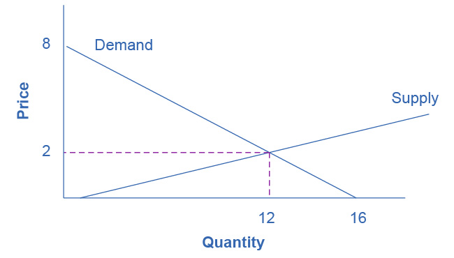


Figure A.2図 A.2
The equations for Qd and Qs are displayed graphically by the sloped lines.
英語のヒント
QdとQsの式を、傾いた直線でグラフに表している。