付録
Exports and Imports as a Function of National Income
英語のヒント
国民所得の関数としての輸出と輸入
The export function, which shows how exports change with the level of a country’s own real GDP, is drawn as a horizontal line, as in the example in Figure D.6 (a) where exports are drawn at a level of $840. Again, as in the case of investment spending and government spending, drawing the export function as horizontal does not imply that exports never change. It just means that they do not change because of what is on the horizontal axis—that is, a country’s own level of domestic production—and instead are shaped by the level of aggregate demand in other countries. More demand for exports from other countries would cause the export function to shift up; less demand for exports from other countries would cause it to shift down.
英語のヒント
輸出関数は、自国の実質GDP水準とともに輸出がどう変わるかを示し、輸出を840ドルに描いた図D.6(a)の例のように水平線となる。ここでも、投資支出や政府支出と同じく、輸出関数を水平に描くことは輸出が決して変化しないという意味ではない。輸出は横軸にある自国の国内生産水準のためには変化せず、他国の総需要水準によって決まるという意味にすぎない。他国から輸出への需要が増えれば輸出関数は上に、減れば下に移動する。
The Export and Import Functions輸出関数と輸入関数
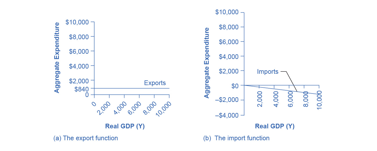
Figure D.6図 D.6
(a) The export function is drawn as a horizontal line because exports are determined by the buying power of other countries and thus do not change with the size of the domestic economy. In this example, exports are set at 840. However, exports can shift up or down, depending on buying patterns in other countries. (b) The import function is drawn in negative territory because expenditures on imported products are a subtraction from expenditures in the domestic economy. In this example, the marginal propensity to import is 0.1, so imports are calculated by multiplying the level of income by –0.1.
英語のヒント
(a)輸出は他国の購買力で決まり、国内経済の大きさでは変化しないため、輸出関数は水平線として描く。この例では輸出は840とする。しかし、他国の購買パターンによって、輸出は上にも下にも動きうる。(b)輸入品への支出は国内経済の支出から差し引くため、輸入関数は負の領域に描く。この例では限界輸入性向は0.1なので、所得水準に-0.1を掛けて輸入を計算する。
Imports are drawn in the Keynesian cross diagram as a downward-sloping line, with the downward slope determined by the marginal propensity to import (MPI), out of national income. In Figure D.6 (b), the marginal propensity to import is 0.1. Thus, if real GDP is $5,000, imports are $500; if national income is $6,000, imports are $600, and so on. The import function is drawn as downward sloping and negative, because it represents a subtraction from the aggregate expenditures in the domestic economy. A change in the marginal propensity to import, perhaps as a result of changes in preferences, would alter the slope of the import function.
英語のヒント
ケインズの交差図では、輸入を右下がりの線として描き、その傾きは国民所得に対する限界輸入性向(MPI)で決まる。図D.6(b)では限界輸入性向は0.1である。したがって実質GDPが5,000ドルなら輸入は500ドル、国民所得が6,000ドルなら輸入は600ドル、といった具合になる。輸入関数は国内経済の総支出からの控除を表すため、右下がりで負に描かれる。たとえば選好の変化によって限界輸入性向が変わると、輸入関数の傾きが変わる。
Building the Combined Aggregate Expenditure Function
英語のヒント
構成要素を合わせた総支出関数の作成
All the components of aggregate demand—consumption, investment, government spending, and the trade balance—are now in place to build the Keynesian cross diagram. Figure D.7 builds up an aggregate expenditure function, based on the numerical illustrations of C, I, G, X, and M that have been used throughout this text. The first three columns in Table D.3 are lifted from the earlier Table D.2, which showed how to bring taxes into the consumption function. The first column is real GDP or national income, which is what appears on the horizontal axis of the income-expenditure diagram. The second column calculates after-tax income, based on the assumption, in this case, that 30% of real GDP is collected in taxes. The third column is based on an MPC of 0.8, so that as after-tax income rises by $700 from one row to the next, consumption rises by $560 (700 × 0.8) from one row to the next. Investment, government spending, and exports do not change with the level of current national income. In the previous discussion, investment was $500, government spending was $1,300, and exports were $840, for a total of $2,640. This total is shown in the fourth column. Imports are 0.1 of real GDP in this example, and the level of imports is calculated in the fifth column. The final column, aggregate expenditures, sums up C + I + G + X – M. This aggregate expenditure line is illustrated in Figure D.7.
英語のヒント
ケインズの交差図を作るための総需要のすべての構成要素、消費、投資、政府支出、貿易収支が揃った。図D.7は、ここまで使ってきたC、I、G、X、Mの数値例に基づいて総支出関数を作る。表D.3の最初の3列は、消費関数に税を組み込む方法を示した先の表D.2から取っている。第1列は実質GDPまたは国民所得で、所得・支出図の横軸に示されるものである。第2列は、この場合は実質GDPの30%を税として徴収するという仮定に基づき、税引後所得を計算する。第3列はMPCを0.8とするので、次の行へ移る際に税引後所得が700ドル増えると、消費は560ドル(700×0.8)増える。投資、政府支出、輸出は、現在の国民所得水準では変化しない。先の議論では投資は500ドル、政府支出は1,300ドル、輸出は840ドルで、合計2,640ドルだった。第4列はこの合計を示す。この例では輸入は実質GDPの0.1で、第5列が輸入水準を計算する。最終列の総支出は、C+I+G+X-Mを合計する。この総支出線を図D.7に示す。
A Keynesian Cross Diagramケインズの交差図
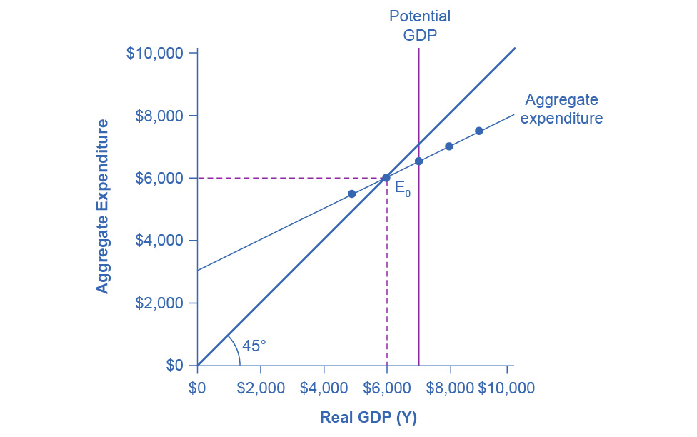


Figure D.7図 D.7
Each combination of national income and aggregate expenditure (after-tax consumption, government spending, investment, exports, and imports) is graphed. The equilibrium occurs where aggregate expenditure is equal to national income; this occurs where the aggregate expenditure schedule crosses the 45-degree line, at a real GDP of $6,000. Potential GDP in this example is $7,000, so the equilibrium is occurring at a level of output or real GDP below the potential GDP level.
英語のヒント
国民所得と総支出(税引後の消費、政府支出、投資、輸出、輸入)の各組み合わせを描く。均衡は総支出が国民所得と等しいところで生じる。総支出曲線が45度線と交わる、実質GDP6,000ドルの点である。この例の潜在GDPは7,000ドルなので、均衡は潜在GDP水準より低い産出量、または実質GDPの水準で生じている。
National Income 国民所得 |
After-Tax Income 税引後所得 |
Consumption 消費 |
Government Spending + Investment + Exports 政府支出+投資+輸出 |
Imports 輸入 |
Aggregate Expenditure 総支出 |
|---|---|---|---|---|---|
$3,000 |
$2,100 |
$2,280 |
$2,640 |
$300 |
$4,620 |
$4,000 |
$2,800 |
$2,840 |
$2,640 |
$400 |
$5,080 |
$5,000 |
$3,500 |
$3,400 |
$2,640 |
$500 |
$5,540 |
$6,000 |
$4,200 |
$3,960 |
$2,640 |
$600 |
$6,000 |
$7,000 |
$4,900 |
$4,520 |
$2,640 |
$700 |
$6,460 |
$8,000 |
$5,600 |
$5,080 |
$2,640 |
$800 |
$6,920 |
$9,000 |
$6,300 |
$5,640 |
$2,640 |
$900 |
$7,380 |
The aggregate expenditure function is formed by stacking on top of each other the consumption function (after taxes), the investment function, the government spending function, the export function, and the import function. The point at which the aggregate expenditure function intersects the vertical axis will be determined by the levels of investment, government, and export expenditures—which do not vary with national income. The upward slope of the aggregate expenditure function will be determined by the marginal propensity to save, the tax rate, and the marginal propensity to import. A higher marginal propensity to save, a higher tax rate, and a higher marginal propensity to import will all make the slope of the aggregate expenditure function flatter—because out of any extra income, more is going to savings or taxes or imports and less to spending on domestic goods and services.
英語のヒント
総支出関数は、消費関数(課税後)、投資関数、政府支出関数、輸出関数、輸入関数を積み重ねて作る。総支出関数が縦軸と交わる点は、国民所得によって変わらない投資、政府、輸出の支出水準によって決まる。総支出関数の右上がりの傾きは、限界貯蓄性向、税率、限界輸入性向によって決まる。限界貯蓄性向、税率、限界輸入性向が高くなると、いずれも総支出関数の傾きは緩やかになる。追加的な所得のうち、貯蓄、税、輸入に回る部分が増え、国内の財・サービスへの支出に回る部分が減るからである。
The equilibrium occurs where national income is equal to aggregate expenditure, which is shown on the graph as the point where the aggregate expenditure schedule crosses the 45-degree line. In this example, the equilibrium occurs at 6,000. This equilibrium can also be read off the table under the figure; it is the level of national income where aggregate expenditure is equal to national income.
英語のヒント
均衡は、国民所得が総支出と等しいところで生じ、グラフでは総支出曲線と45度線の交点として示される。この例では6,000で均衡が生じる。この均衡は図の下の表からも読み取れ、総支出が国民所得と等しくなる国民所得水準である。