付録
We will use graphs more frequently in this book than algebra, but now you know the math behind the graphs.
英語のヒント
本書では代数よりグラフを多く使うが、これでグラフの背後の数学が分かった。
Growth Rates成長率
Growth rates are frequently encountered in real world economics. A growth rate is simply the percentage change in some quantity. It could be your income. It could be a business’s sales. It could be a nation’s GDP. The formula for computing a growth rate is straightforward:
英語のヒント
現実の経済では、成長率によく出会う。成長率は、ある数量の変化率を%で表したものにすぎない。所得、企業の売上、国のGDPなどが対象になる。計算式は単純だ。
Suppose your job pays $10 per hour. Your boss, however, is so impressed with your work that he gives you a $2 per hour raise. The percentage change (or growth rate) in your pay is $2/$10 = 0.20 or 20%.
英語のヒント
時給10ドルの仕事をしているとしよう。上司が仕事ぶりに感心して、時給を2ドル上げてくれた。賃金の変化率、すなわち成長率は2ドル/10ドル=0.20=20%だ。
To compute the growth rate for data over an extended period of time, for example, the average annual growth in GDP over a decade or more, the denominator is commonly defined a little differently. In the previous example, we defined the quantity as the initial quantity—or the quantity when we started. This is fine for a one-time calculation, but when we compute the growth over and over, it makes more sense to define the quantity as the average quantity over the period in question, which is defined as the quantity halfway between the initial quantity and the next quantity. This is harder to explain in words than to show with an example. Suppose a nation’s GDP was $1 trillion in 2005 and $1.03 trillion in 2006. The growth rate between 2005 and 2006 would be the change in GDP ($1.03 trillion – $1.00 trillion) divided by the average GDP between 2005 and 2006 ($1.03 trillion + $1.00 trillion)/2. In other words:
英語のヒント
10年以上のGDPの年平均成長率など、長期間のデータの成長率を計算する際は、分母を少し違う形で定義することが多い。前の例では、数量を最初の値とした。一度だけの計算ならそれでよいが、繰り返し成長率を計算するなら、対象期間の平均値、すなわち最初の値と次の値の中間の数量を使う方が筋が通る。言葉より例で見る方が分かりやすい。ある国のGDPが2005年に1兆ドル、2006年に1.03兆ドルだったとする。この間の成長率は、GDPの変化(1.03兆ドル−1兆ドル)を、両年の平均GDP(1.03兆ドル+1兆ドル)/2で割る。つまり、
Note that if we used the first method, the calculation would be ($1.03 trillion – $1.00 trillion) / $1.00 trillion = 3% growth, which is approximately the same as the second, more complicated method. If you need a rough approximation, use the first method. If you need accuracy, use the second method.
英語のヒント
最初の方法を使うと、(1.03兆ドル−1兆ドル)/1兆ドル=3%成長となり、複雑な2番目の方法とほぼ同じになる。大まかな近似でよければ最初の方法、正確さが必要なら2番目を使おう。
A few things to remember: A positive growth rate means the quantity is growing. A smaller growth rate means the quantity is growing more slowly. A larger growth rate means the quantity is growing more quickly. A negative growth rate means the quantity is decreasing.
英語のヒント
覚えておきたいことがある。正の成長率は数量の増加を意味する。成長率が小さいなら増え方が遅く、大きいなら速い。負の成長率は数量の減少を意味する。
The same change over times yields a smaller growth rate. If you got a $2 raise each year, in the first year the growth rate would be $2/$10 = 20%, as shown above. But in the second year, the growth rate would be $2/$12 = 0.167 or 16.7% growth. In the third year, the same $2 raise would correspond to a $2/$14 = 14.2%. The moral of the story is this: To keep the growth rate the same, the change must increase each period.
英語のヒント
同じ額の変化でも、時がたつと成長率は小さくなる。毎年2ドル昇給すると、最初の年は2ドル/10ドル=20%だが、2年目は2ドル/12ドル=0.167=16.7%、3年目は2ドル/14ドル=14.2%になる。ここから分かるのは、成長率を一定に保つには、毎期の増加額を大きくしなければならないということだ。
Displaying Data Graphically and Interpreting the Graphデータの図示とグラフの解釈
Graphs are also used to display data or evidence. Graphs are a method of presenting numerical patterns. They condense detailed numerical information into a visual form in which relationships and numerical patterns can be seen more easily. For example, which countries have larger or smaller populations? A careful reader could examine a long list of numbers representing the populations of many countries, but with over 200 nations in the world, searching through such a list would take concentration and time. Putting these same numbers on a graph can quickly reveal population patterns. Economists use graphs both for a compact and readable presentation of groups of numbers and for building an intuitive grasp of relationships and connections.
英語のヒント
グラフはデータや証拠の表示にも使う。数値のパターンを示し、詳しい数値情報を視覚的な形にまとめることで、関係や規則性を見やすくする。例えば人口の多い国と少ない国はどこか。多くの国の人口を並べた数値の長い一覧を丁寧に読むこともできるが、世界には200を超える国があり、調べるには集中力と時間が必要だ。同じ数値をグラフにすると、人口のパターンがすぐ分かる。経済学者は、数値の集まりを簡潔で読みやすく示すためにも、関係やつながりを直感的につかむためにもグラフを使う。
Three types of graphs are used in this book: line graphs, pie graphs, and bar graphs. Each is discussed below. We also provide warnings about how graphs can be manipulated to alter viewers’ perceptions of the relationships in the data.
英語のヒント
本書では折れ線グラフ、円グラフ、棒グラフの3種類を使う。以下でそれぞれを説明する。また、データの関係について見る人の認識を変えるため、グラフがどう操作され得るかにも注意を促す。
Line Graphs
英語のヒント
折れ線グラフ
The graphs we have discussed so far are called line graphs, because they show a relationship between two variables: one measured on the horizontal axis and the other measured on the vertical axis.
英語のヒント
ここまで扱ったものは、横軸と縦軸でそれぞれ測る二つの変数の関係を示すため、折れ線グラフと呼ばれる。
Sometimes it is useful to show more than one set of data on the same axes. The data in Table A.2 is displayed in Figure A.3 which shows the relationship between two variables: length and median weight for American baby boys and girls during the first three years of life. (The median means that half of all babies weigh more than this and half weigh less.) The line graph measures length in inches on the horizontal axis and weight in pounds on the vertical axis. For example, point A on the figure shows that a boy who is 28 inches long will have a median weight of about 19 pounds. One line on the graph shows the length-weight relationship for boys and the other line shows the relationship for girls. This kind of graph is widely used by healthcare providers to check whether a child’s physical development is roughly on track.
英語のヒント
The Length-Weight Relationship for American Boys and Girls米国の男女の乳幼児の体長と体重の関係
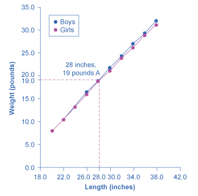
Figure A.3図 A.3
The line graph shows the relationship between height and weight for boys and girls from birth to 3 years. Point A, for example, shows that a boy of 28 inches in height (measured on the horizontal axis) is typically 19 pounds in weight (measured on the vertical axis). These data apply only to children in the first three years of life.
英語のヒント
出生から3歳までの男女の身長と体重の関係を示す。例えば点Aは、身長28インチ(横軸)の男児の体重が、通常19ポンド(縦軸)であることを示す。このデータは生後3年間の子どもだけに当てはまる。
Boys from Birth to 36 Months 出生〜36か月の男児 |
Girls from Birth to 36 Months 出生〜36か月の女児 |
||
|---|---|---|---|
Length (inches) 体長(インチ) |
Weight (pounds) 体重(ポンド) |
Length (inches) 体長(インチ) |
Weight (pounds) 体重(ポンド) |
20.0 |
8.0 |
20.0 |
7.9 |
22.0 |
10.5 |
22.0 |
10.5 |
24.0 |
13.5 |
24.0 |
13.2 |
26.0 |
16.4 |
26.0 |
16.0 |
28.0 |
19.0 |
28.0 |
18.8 |
30.0 |
21.8 |
30.0 |
21.2 |
32.0 |
24.3 |
32.0 |
24.0 |
34.0 |
27.0 |
34.0 |
26.2 |
36.0 |
29.3 |
36.0 |
28.9 |
38.0 |
32.0 |
38.0 |
31.3 |
Not all relationships in economics are linear. Sometimes they are curves. Figure A.4 presents another example of a line graph, representing the data from Table A.3. In this case, the line graph shows how thin the air becomes when you climb a mountain. The horizontal axis of the figure shows altitude, measured in meters above sea level. The vertical axis measures the density of the air at each altitude. Air density is measured by the weight of the air in a cubic meter of space (that is, a box measuring one meter in height, width, and depth). As the graph shows, air pressure is heaviest at ground level and becomes lighter as you climb. Figure A.4 shows that a cubic meter of air at an altitude of 500 meters weighs approximately one kilogram (about 2.2 pounds). However, as the altitude increases, air density decreases. A cubic meter of air at the top of Mount Everest, at about 8,828 meters, would weigh only 0.023 kilograms. The thin air at high altitudes explains why many mountain climbers need to use oxygen tanks as they reach the top of a mountain.
英語のヒント
経済学の関係はすべて直線とは限らず、曲線になることもある。図A.4は表A.3のデータを示す別の折れ線グラフで、山を登ると空気がどれだけ薄くなるかを表す。横軸は海抜高度をメートルで、縦軸は各高度の空気密度を測る。空気密度は、1立方メートル、すなわち高さ・幅・奥行きが各1メートルの箱の中の空気の重さで測る。グラフのように、気圧は地表で最も重く、登るほど軽くなる。図A.4では高度500メートルの空気1立方メートルは約1キログラム、約2.2ポンドだ。高度が増すと空気密度は下がる。約8,828メートルのエベレスト頂上では、空気1立方メートルはわずか0.023キログラムになる。高地の空気が薄いことが、登山者が山頂へ近づくと酸素ボンベを必要とする理由である。
Altitude-Air Density Relationship高度と空気密度の関係
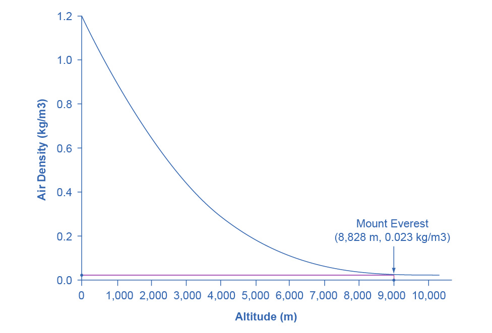
Figure A.4図 A.4
This line graph shows the relationship between altitude, measured in meters above sea level, and air density, measured in kilograms of air per cubic meter. As altitude rises, air density declines. The point at the top of Mount Everest has an altitude of approximately 8,828 meters above sea level (the horizontal axis) and air density of 0.023 kilograms per cubic meter (the vertical axis).
英語のヒント
海抜高度(メートル)と空気密度(1立方メートル当たりのキログラム)の関係。高度が上がると密度が下がる。エベレスト頂上の点は、海抜約8,828メートル(横軸)、空気密度0.023キログラム/立方メートル(縦軸)に位置する。
Altitude (meters) 高度(メートル) |
Air Density (kg/cubic meters) 空気密度(kg/立方メートル) |
|---|---|
0 |
1.200 |
500 |
1.093 |
1,000 |
0.831 |
1,500 |
0.678 |
2,000 |
0.569 |
2,500 |
0.484 |
3,000 |
0.415 |
3,500 |
0.357 |
4,000 |
0.307 |
4,500 |
0.231 |
5,000 |
0.182 |
5,500 |
0.142 |
6,000 |
0.100 |
6,500 |
0.085 |
7,000 |
0.066 |
7,500 |
0.051 |
8,000 |
0.041 |
8,500 |
0.025 |
9,000 |
0.022 |
9,500 |
0.019 |
10,000 |
0.014 |
The length-weight relationship and the altitude-air density relationships in these two figures represent averages. If you were to collect actual data on air pressure at different altitudes, the same altitude in different geographic locations will have slightly different air density, depending on factors like how far you are from the equator, local weather conditions, and the humidity in the air. Similarly, in measuring the height and weight of children for the previous line graph, children of a particular height would have a range of different weights, some above average and some below. In the real world, this sort of variation in data is common. The task of a researcher is to organize that data in a way that helps to understand typical patterns. The study of statistics, especially when combined with computer statistics and spreadsheet programs, is a great help in organizing this kind of data, plotting line graphs, and looking for typical underlying relationships. For most economics and social science majors, a statistics course will be required at some point.
英語のヒント
二つの図の体長・体重と高度・空気密度の関係は、平均を表す。各高度の実際の気圧を調べると、同じ高度でも、赤道からの距離、現地の天候、湿度などによって密度は多少異なる。同様に、同じ身長の子どもの体重にも幅があり、平均より重い子も軽い子もいる。現実のデータには、このようなばらつきが普通にある。研究者の仕事は、典型的なパターンを理解できるようデータを整理することだ。統計学、とりわけ統計ソフトや表計算ソフトを組み合わせた分析は、データ整理、折れ線グラフの作成、背後の典型的な関係の探索に役立つ。経済学や社会科学の専攻では、多くの場合、どこかで統計の履修が必要になる。
One common line graph is called a time series, in which the horizontal axis shows time and the vertical axis displays another variable. Thus, a time series graph shows how a variable changes over time. Figure A.5 shows the unemployment rate in the United States since 1975, where unemployment is defined as the percentage of adults who want jobs and are looking for a job, but cannot find one. The points for the unemployment rate in each year are plotted on the graph, and a line then connects the points, showing how the unemployment rate has moved up and down since 1975. The line graph makes it easy to see, for example, that the highest unemployment rate during this time period was slightly less than 10% in the early 1980s and 2010, while the unemployment rate declined from the early 1990s to the end of the 1990s, before rising and then falling back in the early 2000s, and then rising sharply during the recession from 2008–2009.
英語のヒント
よく使う折れ線グラフに時系列がある。横軸に時間、縦軸に別の変数を取り、時間とともに変数がどう変わるかを示す。図A.5は1975年以降の米国の失業率で、仕事を望んで探しているが見つからない成人の割合と定義する。各年の失業率の点を線で結び、1975年以降の上下を示す。例えば、この期間で最も高い失業率は1980年代初めと2010年の10%弱であることがすぐ分かる。1990年代初めから末にかけて下がり、2000年代初めに上昇後再び低下し、2008〜2009年の景気後退で急上昇したことも見て取れる。
U.S. Unemployment Rate, 1975–2014米国の失業率、1975〜2014年
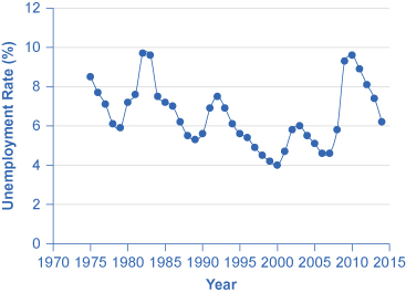


Figure A.5図 A.5
This graph provides a quick visual summary of unemployment data. With a graph like this, it is easy to spot the times of high unemployment and of low unemployment.
英語のヒント
失業データを視覚的に素早く把握できるグラフ。失業率の高い時期と低い時期を容易に見つけられる。