付録
Pie Graphs
英語のヒント
円グラフ
A pie graph (sometimes called a pie chart) is used to show how an overall total is divided into parts. A circle represents a group as a whole. The slices of this circular “pie” show the relative sizes of subgroups.
英語のヒント
円グラフは、全体がどう分かれているかを示す。円が集団全体を表し、円形の「パイ」の切片が各下位集団の相対的な大きさを表す。
Figure A.6 shows how the U.S. population was divided among children, working age adults, and the elderly in 1970, 2000, and what is projected for 2030. The information is first conveyed with numbers in Table A.4, and then in three pie charts. The first column of Table A.4 shows the total U.S. population for each of the three years. Columns 2–4 categorize the total in terms of age groups—from birth to 18 years, from 19 to 64 years, and 65 years and above. In columns 2–4, the first number shows the actual number of people in each age category, while the number in parentheses shows the percentage of the total population comprised by that age group.
英語のヒント
Year 年 |
Total Population 総人口 |
19 and Under 19歳以下 |
20–64 years 20〜64歳 |
Over 65 65歳超 |
|---|---|---|---|---|
1970 |
205.0 million 2億500万人 |
77.2 (37.6%) |
107.7 (52.5%) |
20.1 (9.8%) |
2000 |
275.4 million 2億7,540万人 |
78.4 (28.5%) |
162.2 (58.9%) |
34.8 (12.6%) |
2030 |
351.1 million 3億5,110万人 |
92.6 (26.4%) |
188.2 (53.6%) |
70.3 (20.0%) |
Pie Graphs of the U.S. Age Distribution (numbers in millions)米国の年齢分布の円グラフ(単位:百万人)
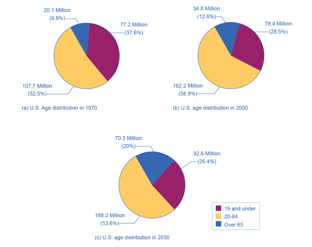
Figure A.6図 A.6
The three pie graphs illustrate the division of total population into three age groups for the three different years.
英語のヒント
3枚の円グラフが、3か年の総人口をそれぞれ三つの年齢層に分けて示す。
In a pie graph, each slice of the pie represents a share of the total, or a percentage. For example, 50% would be half of the pie and 20% would be one-fifth of the pie. The three pie graphs in Figure A.6 show that the share of the U.S. population 65 and over is growing. The pie graphs allow you to get a feel for the relative size of the different age groups from 1970 to 2000 to 2030, without requiring you to slog through the specific numbers and percentages in the table. Some common examples of how pie graphs are used include dividing the population into groups by age, income level, ethnicity, religion, occupation; dividing different firms into categories by size, industry, number of employees; and dividing up government spending or taxes into its main categories.
英語のヒント
円グラフの各切片は、全体に占める割合を表す。50%なら半円、20%なら5分の1だ。図A.6の3枚のグラフから、米国で65歳以上の割合が増えていることが分かる。表の細かな人数や割合を一つずつ追わなくても、1970年、2000年、2030年の各年齢層の相対的な大きさをつかめる。よくある用途には、人口を年齢・所得・民族・宗教・職業で分けること、企業を規模・産業・従業員数で分類すること、政府の支出や税収を主要項目に分けることがある。
Bar Graphs
英語のヒント
棒グラフ
A bar graph uses the height of different bars to compare quantities. Table A.5 lists the 12 most populous countries in the world. Figure A.7 provides this same data in a bar graph. The height of the bars corresponds to the population of each country. Although you may know that China and India are the most populous countries in the world, seeing how the bars on the graph tower over the other countries helps illustrate the magnitude of the difference between the sizes of national populations.
英語のヒント
Leading Countries of the World by Population, 2015 (in millions)世界の人口上位国、2015年(単位:百万人)
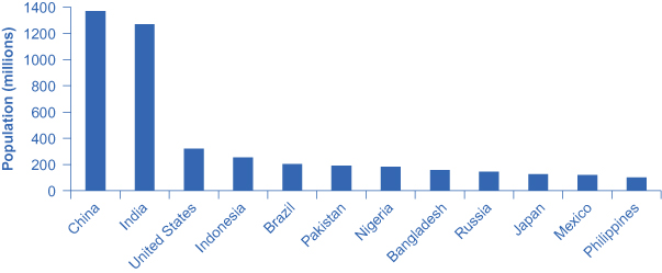
Figure A.7図 A.7
The graph shows the 12 countries of the world with the largest populations. The height of the bars in the bar graph shows the size of the population for each country.
英語のヒント
世界で人口の多い12か国を示す。各国の人口の大きさを棒の高さで表す。
Country 国 |
Population 人口 |
|---|---|
China 中国 |
1,369 |
India インド |
1,270 |
United States 米国 |
321 |
Indonesia インドネシア |
255 |
Brazil ブラジル |
204 |
Pakistan パキスタン |
190 |
Nigeria ナイジェリア |
184 |
Bangladesh バングラデシュ |
158 |
Russia ロシア |
146 |
Japan 日本 |
127 |
Mexico メキシコ |
121 |
Philippines フィリピン |
101 |
Bar graphs can be subdivided in a way that reveals information similar to that we can get from pie charts. Figure A.8 offers three bar graphs based on the information from Figure A.6 about the U.S. age distribution in 1970, 2000, and 2030. Figure A.8 (a) shows three bars for each year, representing the total number of persons in each age bracket for each year. Figure A.8 (b) shows just one bar for each year, but the different age groups are now shaded inside the bar. In Figure A.8 (c), still based on the same data, the vertical axis measures percentages rather than the number of persons. In this case, all three bar graphs are the same height, representing 100% of the population, with each bar divided according to the percentage of population in each age group. It is sometimes easier for a reader to run their eyes across several bar graphs, comparing the shaded areas, rather than trying to compare several pie graphs.
英語のヒント
U.S. Population with Bar Graphs棒グラフで見る米国の人口
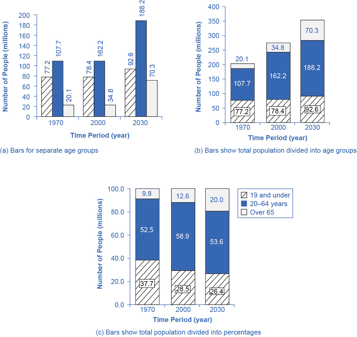
Figure A.8図 A.8
Population data can be represented in different ways. (a) Shows three bars for each year, representing the total number of persons in each age bracket for each year. (b) Shows just one bar for each year, but the different age groups are now shaded inside the bar. (c) Sets the vertical axis as a measure of percentages rather than the number of persons. All three bar graphs are the same height and each bar is divided according to the percentage of population in each age group.
英語のヒント
人口データはさまざまに表せる。(a)は各年3本の棒で年齢層ごとの人数を示す。(b)は各年1本の棒の中を年齢層ごとに色分けする。(c)は縦軸を人数でなく割合とし、3本とも同じ高さで、各棒を年齢層の人口割合に応じて分ける。
Figure A.7 and Figure A.8 show how the bars can represent countries or years, and how the vertical axis can represent a numerical or a percentage value. Bar graphs can also compare size, quantity, rates, distances, and other quantitative categories.
英語のヒント
Comparing Line Graphs with Pie Charts and Bar Graphs
英語のヒント
折れ線・円・棒グラフの比較
Now that you are familiar with pie graphs, bar graphs, and line graphs, how do you know which graph to use for your data? Pie graphs are often better than line graphs at showing how an overall group is divided. However, if a pie graph has too many slices, it can become difficult to interpret.
英語のヒント
3種類のグラフが分かったところで、自分のデータにどれを使えばよいだろうか。全体の内訳を示すには、円グラフが折れ線より適していることが多い。しかし、切片が多すぎると解釈しにくくなる。
Bar graphs are especially useful when comparing quantities. For example, if you are studying the populations of different countries, as in Figure A.7, bar graphs can show the relationships between the population sizes of multiple countries. Not only can it show these relationships, but it can also show breakdowns of different groups within the population.
英語のヒント
棒グラフは数量の比較に特に役立つ。図A.7のように各国の人口を調べるなら、国同士の人口規模の関係を示せる。それだけでなく、人口内部の集団別の内訳も示せる。
A line graph is often the most effective format for illustrating a relationship between two variables that are both changing. For example, time series graphs can show patterns as time changes, like the unemployment rate over time. Line graphs are widely used in economics to present continuous data about prices, wages, quantities bought and sold, the size of the economy.
英語のヒント
両方とも変わる二つの変数の関係を示すには、折れ線グラフが最も効果的なことが多い。例えば、時系列グラフは時間とともに失業率などが変わる様子を示す。経済学では、価格、賃金、売買量、経済規模などの連続的なデータに広く使う。
How Graphs Can Be Misleading
英語のヒント
グラフが誤解を招く仕組み
Graphs not only reveal patterns; they can also alter how patterns are perceived. To see some of the ways this can be done, consider the line graphs of Figure A.9, Figure A.10, and Figure A.11. These graphs all illustrate the unemployment rate—but from different perspectives.
英語のヒント
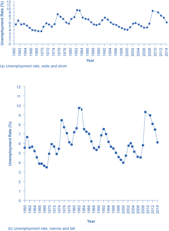
Figure A.9図 A.9
Presenting Unemployment Rates in Different Ways, All of Them Accurate失業率のさまざまな示し方――どれも正確
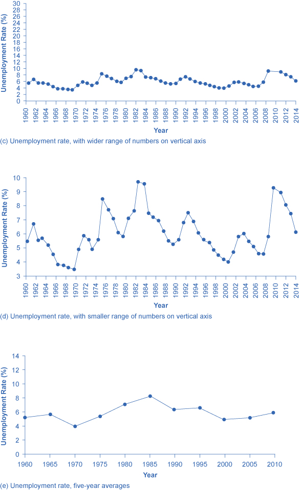
Figure A.10図 A.10
Simply changing the width and height of the area in which data is displayed can alter the perception of the data.
英語のヒント
データを表示する領域の幅と高さを変えるだけで、受ける印象が変わる。
Presenting Unemployment Rates in Different Ways, All of Them Accurate失業率のさまざまな示し方――どれも正確
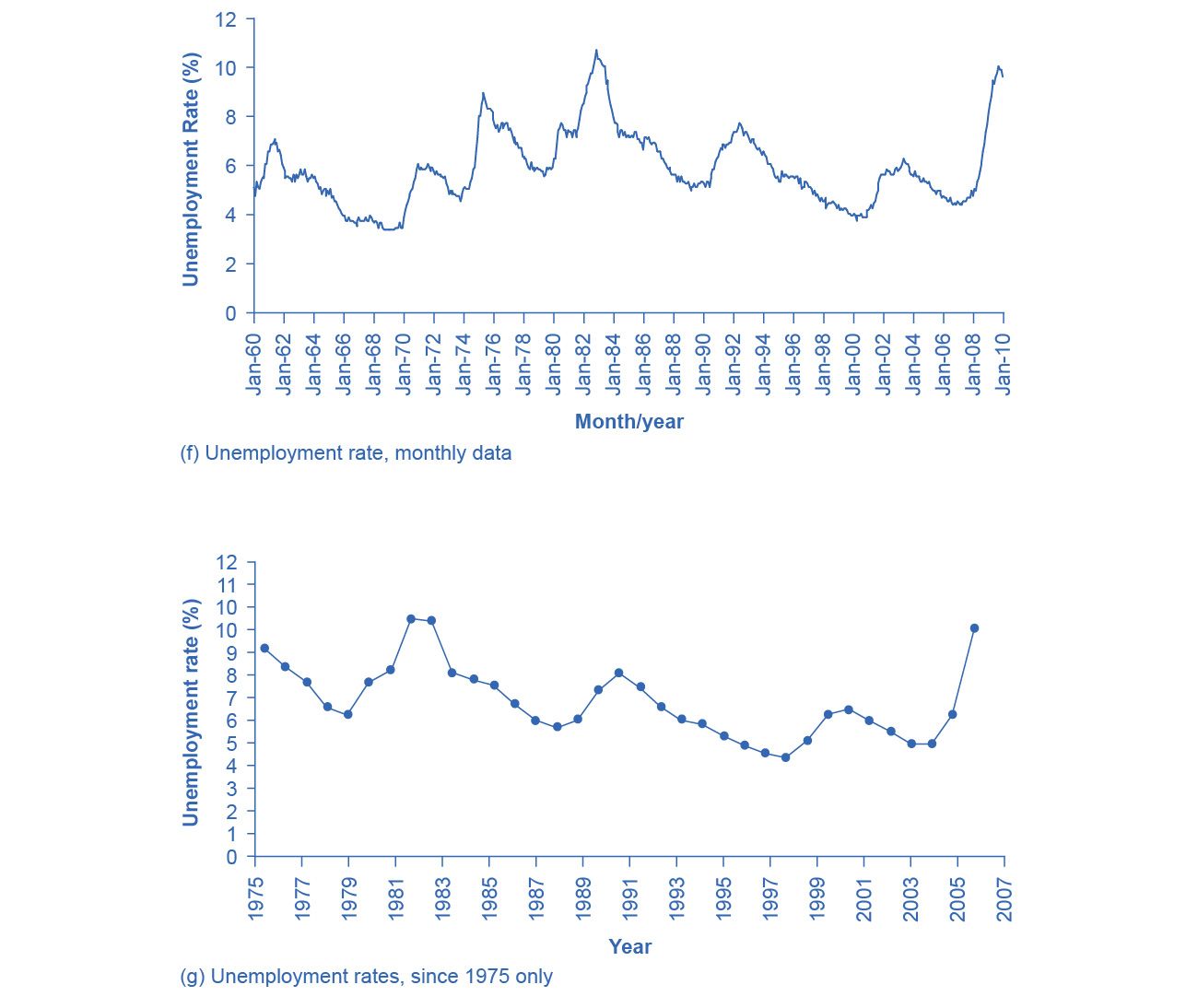


Figure A.11図 A.11
Simply changing the width and height of the area in which data is displayed can alter the perception of the data.
英語のヒント
データを表示する領域の幅と高さを変えるだけで、受ける印象が変わる。
Suppose you wanted a graph which gives the impression that the rise in unemployment in 2009 was not all that large, or all that extraordinary by historical standards. You might choose to present your data as in Figure A.9 (a). Figure A.9 (a) includes much of the same data presented earlier in Figure A.5, but stretches the horizontal axis out longer relative to the vertical axis. By spreading the graph wide and flat, the visual appearance is that the rise in unemployment is not so large, and is similar to some past rises in unemployment. Now imagine you wanted to emphasize how unemployment spiked substantially higher in 2009. In this case, using the same data, you can stretch the vertical axis out relative to the horizontal axis, as in Figure A.9 (b), which makes all rises and falls in unemployment appear larger.
英語のヒント
A similar effect can be accomplished without changing the length of the axes, but by changing the scale on the vertical axis. In Figure A.10 (c), the scale on the vertical axis runs from 0% to 30%, while in Figure A.10 (d), the vertical axis runs from 3% to 10%. Compared to Figure A.5, where the vertical scale runs from 0% to 12%, Figure A.10 (c) makes the fluctuation in unemployment look smaller, while Figure A.10 (d) makes it look larger.
英語のヒント
Another way to alter the perception of the graph is to reduce the amount of variation by changing the number of points plotted on the graph. Figure A.10 (e) shows the unemployment rate according to five-year averages. By averaging out some of the year-to-year changes, the line appears smoother and with fewer highs and lows. In reality, the unemployment rate is reported monthly, and Figure A.11 (f) shows the monthly figures since 1960, which fluctuate more than the five-year average. Figure A.11 (f) is also a vivid illustration of how graphs can compress lots of data. The graph includes monthly data since 1960, which over almost 50 years, works out to nearly 600 data points. Reading that list of 600 data points in numerical form would be hypnotic. You can, however, get a good intuitive sense of these 600 data points very quickly from the graph.
英語のヒント
A final trick in manipulating the perception of graphical information is that, by choosing the starting and ending points carefully, you can influence the perception of whether the variable is rising or falling. The original data show a general pattern with unemployment low in the 1960s, but spiking up in the mid-1970s, early 1980s, early 1990s, early 2000s, and late 2000s. Figure A.11 (g), however, shows a graph that goes back only to 1975, which gives an impression that unemployment was more-or-less gradually falling over time until the 2009 recession pushed it back up to its “original” level—which is a plausible interpretation if one starts at the high point around 1975.
英語のヒント
最後の手法は、始点と終点を注意深く選び、変数が上昇しているか下降しているかの印象に影響を与えることだ。元のデータは、1960年代に失業率が低く、1970年代半ば、1980年代初め、1990年代初め、2000年代初めと末に急上昇する全体像を示す。しかし図A.11(g)は1975年までしか遡らない。そのため、失業率がおおむね徐々に低下し、2009年の景気後退で「元の」水準へ押し戻された印象になる。1975年頃の高い点から始めるなら、これはもっともらしい解釈だ。
These kinds of tricks—or shall we just call them “presentation choices”— are not limited to line graphs. In a pie chart with many small slices and one large slice, someone must decide what categories should be used to produce these slices in the first place, thus making some slices appear bigger than others. If you are making a bar graph, you can make the vertical axis either taller or shorter, which will tend to make variations in the height of the bars appear more or less.
英語のヒント
こうした手法、あるいは単に「表示上の選択」は、折れ線に限らない。小さな切片が多く大きな切片が一つある円グラフでは、そもそもどの分類を使うかを誰かが決めることで、一部をほかより大きく見せている。棒グラフでも、縦軸を長くしたり短くしたりすると、棒の高さのばらつきが大きくも小さくも見える。
Being able to read graphs is an essential skill, both in economics and in life. A graph is just one perspective or point of view, shaped by choices such as those discussed in this section. Do not always believe the first quick impression from a graph. View with caution.
英語のヒント
グラフを読めることは、経済学でも日常生活でも欠かせない。グラフは、この節で述べたような選択で形作られた一つの視点にすぎない。最初に受けた印象をいつも信じてはいけない。注意して見よう。