付録
Building the Aggregate Expenditure Schedule総支出曲線の作成
Aggregate expenditure is the key to the expenditure-income model. The aggregate expenditure schedule shows, either in the form of a table or a graph, how aggregate expenditures in the economy rise as real GDP or national income rises. Thus, in thinking about the components of the aggregate expenditure line—consumption, investment, government spending, exports and imports—the key question is how expenditures in each category will adjust as national income rises.
英語のヒント
総支出は、支出・所得モデルの鍵である。総支出曲線は表またはグラフで、実質GDPや国民所得が増えるにつれて経済の総支出がどう増えるかを示す。したがって、総支出線の構成要素である消費、投資、政府支出、輸出、輸入を考える際の重要な問いは、国民所得の増加に対し、それぞれの区分の支出がどう調整されるかである。
Consumption as a Function of National Income
英語のヒント
国民所得の関数としての消費
How do consumption expenditures increase as national income rises? People can do two things with their income: consume it or save it (for the moment, let’s ignore the need to pay taxes with some of it). Each person who receives an additional dollar faces this choice. The marginal propensity to consume (MPC), is the share of the additional dollar of income a person decides to devote to consumption expenditures. The marginal propensity to save (MPS) is the share of the additional dollar a person decides to save. It must always hold true that:
英語のヒント
国民所得が増えると、消費支出はどのように増えるだろうか。人々は所得を消費するか貯蓄するかの二つに使える(今は一部を納税に使う必要を無視しよう)。追加の1ドルを受け取る人は、誰もがこの選択に直面する。限界消費性向(MPC)は、追加的な所得1ドルのうち、消費支出に回すことを決める割合である。限界貯蓄性向(MPS)は、追加の1ドルのうち貯蓄すると決める割合である。次の関係が常に成立しなければならない。
For example, if the marginal propensity to consume out of the marginal amount of income earned is 0.9, then the marginal propensity to save is 0.1.
英語のヒント
たとえば、追加で得た所得に対する限界消費性向が0.9なら、限界貯蓄性向は0.1である。
With this relationship in mind, consider the relationship among income, consumption, and savings shown in Figure D.2. (Note that we use “Aggregate Expenditure” on the vertical axis in this and the following figures, because all consumption expenditures are parts of aggregate expenditures.)
英語のヒント
この関係を念頭に、図D.2に示す所得、消費、貯蓄の関係を考えよう。(消費支出はすべて総支出の一部なので、この図と以下の図では縦軸を「総支出」としている点に注意しよう。)
An assumption commonly made in this model is that even if income were zero, people would have to consume something. In this example, consumption would be $600 even if income were zero. Then, the MPC is 0.8 and the MPS is 0.2. Thus, when income increases by $1,000, consumption rises by $800 and savings rises by $200. At an income of $4,000, total consumption will be the $600 that would be consumed even without any income, plus $4,000 multiplied by the marginal propensity to consume of 0.8, or $ 3,200, for a total of $ 3,800. The total amount of consumption and saving must always add up to the total amount of income. (Exactly how a situation of zero income and negative savings would work in practice is not important, because even low-income societies are not literally at zero income, so the point is hypothetical.) This relationship between income and consumption, illustrated in Figure D.2 and Table D.1, is called the consumption function.
英語のヒント
このモデルでよく置かれる仮定は、所得がゼロでも、人々は何かを消費しなければならないというものである。この例では、所得がゼロでも消費は600ドルとなる。そしてMPCは0.8、MPSは0.2である。したがって、所得が1,000ドル増えると、消費は800ドル、貯蓄は200ドル増える。所得4,000ドルでは、総消費は、所得がなくても消費される600ドルに、4,000ドルに限界消費性向0.8を掛けた3,200ドルを加え、3,800ドルとなる。消費と貯蓄の総額は、常に所得の総額と等しくなければならない。(所得ゼロで貯蓄が負という状況が実際にどう成り立つかは重要でない。低所得の社会でも文字どおり所得がゼロではなく、この点は仮想的だからである。)図D.2と表D.1が示すこの所得と消費の関係を、消費関数と呼ぶ。
The Consumption Function消費関数
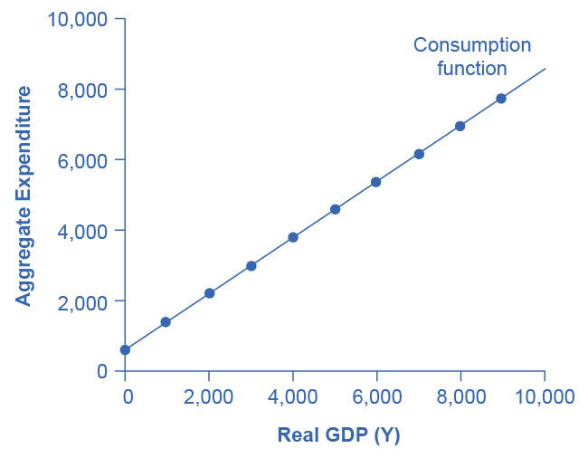
Figure D.2図 D.2
In the expenditure-output model, how does consumption increase with the level of national income? Output on the horizontal axis is conceptually the same as national income, since the value of all final output that is produced and sold must be income to someone, somewhere in the economy. At a national income level of zero, $600 is consumed. Then, each time income rises by $1,000, consumption rises by $800, because in this example, the marginal propensity to consume is 0.8.
英語のヒント
支出・産出モデルで、国民所得の水準とともに消費はどう増えるだろうか。生産・販売される最終生産物の価値は、経済のどこかで誰かの所得になるので、横軸の産出量は概念上、国民所得と同じである。国民所得がゼロでも600ドルが消費される。その後、所得が1,000ドル増えるたびに消費は800ドル増える。この例では限界消費性向が0.8だからである。
The pattern of consumption shown in Table D.1 is plotted in Figure D.2. To calculate consumption, multiply the income level by 0.8, for the marginal propensity to consume, and add $600, for the amount that would be consumed even if income was zero. Consumption plus savings must be equal to income.
英語のヒント
Income 所得 |
Consumption 消費 |
Savings 貯蓄 |
|---|---|---|
$0 |
$600 |
–$600 |
$1,000 |
$1,400 |
–$400 |
$2,000 |
$2,200 |
–$200 |
$3,000 |
$3,000 |
$0 |
$4,000 |
$3,800 |
$200 |
$5,000 |
$4,600 |
$400 |
$6,000 |
$5,400 |
$600 |
$7,000 |
$6,200 |
$800 |
$8,000 |
$7,000 |
$1,000 |
$9,000 |
$7,800 |
$1,200 |
However, a number of factors other than income can also cause the entire consumption function to shift. These factors were summarized in the earlier discussion of consumption, and listed in Table D.1. When the consumption function moves, it can shift in two ways: either the entire consumption function can move up or down in a parallel manner, or the slope of the consumption function can shift so that it becomes steeper or flatter. For example, if a tax cut leads consumers to spend more, but does not affect their marginal propensity to consume, it would cause an upward shift to a new consumption function that is parallel to the original one. However, a change in household preferences for saving that reduced the marginal propensity to save would cause the slope of the consumption function to become steeper: that is, if the savings rate is lower, then every increase in income leads to a larger rise in consumption.
英語のヒント
しかし、所得以外のさまざまな要因も、消費関数全体を移動させる。これらの要因は、先の消費の議論で要約され、表D.1に列挙された。消費関数の移動には二つの形がある。全体が平行に上または下へ動く場合と、傾きが変わって急または緩やかになる場合である。たとえば、減税で消費者が支出を増やしても限界消費性向は変わらなければ、消費関数は元の関数と平行な新しい関数へ上方移動する。しかし、貯蓄に対する家計の選好が変わり、限界貯蓄性向が低くなると、消費関数の傾きは急になる。つまり、貯蓄率が低ければ、所得が増えるたびに消費がより大きく増える。
Investment as a Function of National Income
英語のヒント
国民所得の関数としての投資
Investment decisions are forward-looking, based on expected rates of return. Precisely because investment decisions depend primarily on perceptions about future economic conditions, they do not depend primarily on the level of GDP in the current year. Thus, on a Keynesian cross diagram, the investment function can be drawn as a horizontal line, at a fixed level of expenditure. Figure D.3 shows an investment function where the level of investment is, for the sake of concreteness, set at the specific level of 500. Just as a consumption function shows the relationship between consumption levels and real GDP (or national income), the investment function shows the relationship between investment levels and real GDP.
英語のヒント
投資の意思決定は、予想収益率に基づいて将来を見据えるものである。投資の意思決定は主に将来の経済状況の見通しに依存するため、まさにその理由で、当年のGDP水準には主に依存しない。したがって、ケインズの交差図では、投資関数を一定の支出水準の水平線として描ける。図D.3は、具体性のために投資水準を500に設定した投資関数を示す。消費関数が消費水準と実質GDP、または国民所得の関係を示すのと同じく、投資関数は投資水準と実質GDPの関係を示す。
The Investment Function投資関数
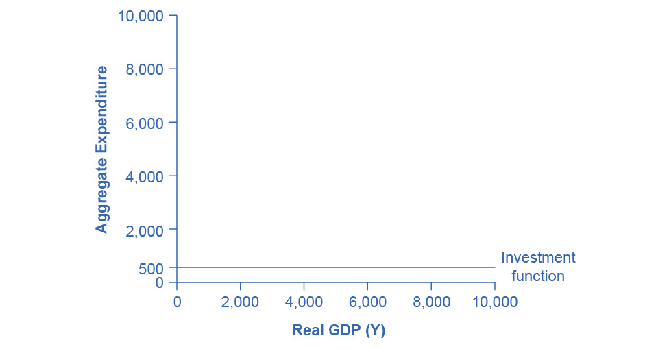
Figure D.3図 D.3
The investment function is drawn as a flat line because investment is based on interest rates and expectations about the future, and so it does not change with the level of current national income. In this example, investment expenditures are at a level of 500. However, changes in factors like technological opportunities, expectations about near-term economic growth, and interest rates would all cause the investment function to shift up or down.
英語のヒント
投資は利子率と将来への予想に基づき、現在の国民所得の水準によって変わらないため、投資関数は水平線として描く。この例では投資支出は500である。しかし、技術的な機会、近い将来の経済成長への予想、利子率などの要因の変化は、いずれも投資関数を上または下へ移動させる。
The appearance of the investment function as a horizontal line does not mean that the level of investment never moves. It means only that in the context of this two-dimensional diagram, the level of investment on the vertical aggregate expenditure axis does not vary according to the current level of real GDP on the horizontal axis. However, all the other factors that vary investment—new technological opportunities, expectations about near-term economic growth, interest rates, the price of key inputs, and tax incentives for investment—can cause the horizontal investment function to shift up or down.
英語のヒント
投資関数が水平線で示されることは、投資水準が決して動かないという意味ではない。この二次元の図では、縦の総支出軸上の投資水準が、横軸の現在の実質GDP水準に応じては変化しない、という意味にすぎない。しかし、新たな技術的機会、近い将来の経済成長への予想、利子率、主要な投入物の価格、投資への税制上の誘因など、投資を変える他のすべての要因は、水平な投資関数を上または下へ移動させうる。
Government Spending and Taxes as a Function of National Income
英語のヒント
国民所得の関数としての政府支出と税
In the Keynesian cross diagram, government spending appears as a horizontal line, as in Figure D.4, where government spending is set at a level of 1,300. As in the case of investment spending, this horizontal line does not mean that government spending is unchanging. It means only that government spending changes when Congress decides on a change in the budget, rather than shifting in a predictable way with the current size of the real GDP shown on the horizontal axis.
英語のヒント
ケインズの交差図では、政府支出を1,300に設定した図D.4のように、政府支出は水平線として現れる。投資支出と同じく、この水平線は政府支出が変化しないことを意味しない。政府支出は、横軸に示す現在の実質GDPの大きさに応じて予測可能な形で変化するのではなく、議会が予算の変更を決めたときに変わる、という意味にすぎない。
The Government Spending Function政府支出関数
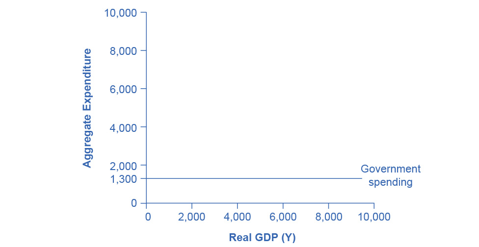
Figure D.4図 D.4
The level of government spending is determined by political factors, not by the level of real GDP in a given year. Thus, government spending is drawn as a horizontal line. In this example, government spending is at a level of 1,300. Congressional decisions to increase government spending will cause this horizontal line to shift up, while decisions to reduce spending would cause it to shift down.
英語のヒント
政府支出の水準は、その年の実質GDP水準ではなく、政治的要因によって決まる。そのため、政府支出は水平線として描く。この例では政府支出は1,300である。議会が政府支出の増加を決めれば、この水平線は上に動き、支出の削減を決めれば下に動く。
The situation of taxes is different because taxes often rise or fall with the volume of economic activity. For example, income taxes are based on the level of income earned and sales taxes are based on the amount of sales made, and both income and sales tend to be higher when the economy is growing and lower when the economy is in a recession. For the purposes of constructing the basic Keynesian cross diagram, it is helpful to view taxes as a proportionate share of GDP. In the United States, for example, taking federal, state, and local taxes together, government typically collects about 30–35 % of income as taxes.
英語のヒント
税は、経済活動の量とともに増減することが多いため、事情が異なる。たとえば、所得税は得られる所得の水準に、売上税は販売額に基づき、所得も売上も経済成長時には増え、景気後退時には減る傾向がある。基本的なケインズの交差図を作るには、税をGDPの一定割合と捉えると便利である。たとえば米国では、連邦・州・地方の税を合わせると、政府は通常、所得の約30~35%を税として徴収する。
Table D.2 revises the earlier table on the consumption function so that it takes taxes into account. The first column shows national income. The second column calculates taxes, which in this example are set at a rate of 30%, or 0.3. The third column shows after-tax income; that is, total income minus taxes. The fourth column then calculates consumption in the same manner as before: multiply after-tax income by 0.8, representing the marginal propensity to consume, and then add $600, for the amount that would be consumed even if income was zero. When taxes are included, the marginal propensity to consume is reduced by the amount of the tax rate, so each additional dollar of income results in a smaller increase in consumption than before taxes. For this reason, the consumption function, with taxes included, is flatter than the consumption function without taxes, as Figure D.5 shows.
英語のヒント
The Consumption Function Before and After Taxes課税前後の消費関数
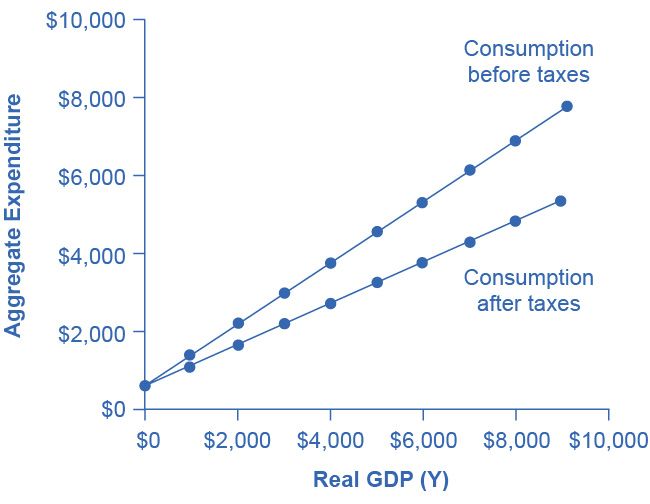


Figure D.5図 D.5
The upper line repeats the consumption function from Figure D.2. The lower line shows the consumption function if taxes must first be paid on income, and then consumption is based on after-tax income.
英語のヒント
上の線は、図D.2の消費関数を再掲したものである。下の線は、まず所得から税を払い、その後の税引後所得に基づいて消費する場合の消費関数を示す。
Income 所得 |
Taxes 税 |
After-Tax Income 税引後所得 |
Consumption 消費 |
Savings 貯蓄 |
|---|---|---|---|---|
$0 |
$0 |
$0 |
$600 |
–$600 |
$1,000 |
$300 |
$700 |
$1,160 |
–$460 |
$2,000 |
$600 |
$1,400 |
$1,720 |
–$320 |
$3,000 |
$900 |
$2,100 |
$2,280 |
–$180 |
$4,000 |
$1,200 |
$2,800 |
$2,840 |
–$40 |
$5,000 |
$1,500 |
$3,500 |
$3,400 |
$100 |
$6,000 |
$1,800 |
$4,200 |
$3,960 |
$240 |
$7,000 |
$2,100 |
$4,900 |
$4,520 |
$380 |
$8,000 |
$2,400 |
$5,600 |
$5,080 |
$520 |
$9,000 |
$2,700 |
$6,300 |
$5,640 |
$660 |