第24章総需要・総供給モデル
24.3 Shifts in Aggregate Supply24.3 総供給のシフト
Learning Objectives学習目標
Learning Objectives学習目標
By the end of this section, you will be able to:
英語のヒント
この節を学ぶと、次のことができるようになる。
- Explain how productivity growth changes the aggregate supply curve
英語のヒント
生産性の向上が総供給曲線をどう変えるか説明する - Explain how changes in input prices change the aggregate supply curve
英語のヒント
投入価格の変化が総供給曲線をどう変えるか説明する
The original equilibrium in the AD/AS diagram will shift to a new equilibrium if the AS or AD curve shifts. When the aggregate supply curve shifts to the right, then at every price level, producers supply a greater quantity of real GDP. When the AS curve shifts to the left, then at every price level, producers supply a lower quantity of real GDP. This module discusses two of the most important factors that can lead to shifts in the AS curve: productivity growth and changes in input prices.
英語のヒント
AS曲線またはAD曲線がシフトすると、AD/AS図の元の均衡は新しい均衡へ移る。総供給曲線が右へシフトすると、すべての物価水準で、生産者はより多くの実質GDPを供給する。AS曲線が左へシフトすると、すべての物価水準で、生産者はより少ない実質GDPを供給する。本節では、AS曲線をシフトさせる最も重要な要因のうち、生産性の向上と投入価格の変化の二つを論じる。
How Productivity Growth Shifts the AS Curve生産性の向上はAS曲線をどうシフトさせるか
In the long run, the most important factor shifting the AS curve is productivity growth. Productivity means how much output can be produced with a given quantity of labor. One measure of this is output per worker or GDP per capita. Over time, productivity grows so that the same quantity of labor can produce more output. Historically, the real growth in GDP per capita in an advanced economy like the United States has averaged about 2% to 3% per year, but productivity growth has been faster during certain extended periods like the 1960s and the late 1990s through the early 2000s, or slower during periods like the 1970s. A higher level of productivity shifts the AS curve to the right, because with improved productivity, firms can produce a greater quantity of output at every price level. Figure 24.7 (a) shows an outward shift in productivity over two time periods. The AS curve shifts out from SRAS0 to SRAS1 to SRAS2, and the equilibrium shifts from E0 to E1 to E2. Note that with increased productivity, workers can produce more GDP. Thus, full employment corresponds to a higher level of potential GDP, which we show as a rightward shift in LRAS from LRAS0 to LRAS1 to LRAS2.
英語のヒント
長期にAS曲線をシフトさせる最も重要な要因は、生産性の向上である。生産性とは、一定量の労働でどれだけの生産物を生み出せるかを意味する。その一つの尺度は、労働者1人当たり生産、または1人当たりGDPである。時間とともに生産性が高まると、同じ量の労働でより多く生産できる。歴史的に、米国のような先進経済の1人当たり実質GDP成長率は年平均約2~3%であった。しかし、1960年代や1990年代後半から2000年代初めのような一定の長い期間には生産性の伸びが速く、1970年代のような期間には遅かった。生産性が向上すると、すべての物価水準で企業がより多く生産できるため、AS曲線は右へシフトする。図24.7(a)は、二つの期間にわたる生産性の外側へのシフトを示す。AS曲線はSRAS0からSRAS1へ、さらにSRAS2へと外へシフトし、均衡はE0からE1へ、さらにE2へ移る。生産性が高まると、労働者がより多くのGDPを生産できることに注目しよう。したがって、完全雇用はより高い潜在GDP水準に対応する。これはLRAS0からLRAS1へ、さらにLRAS2への、LRASの右方シフトで示される。
Shifts in Aggregate Supply総供給のシフト
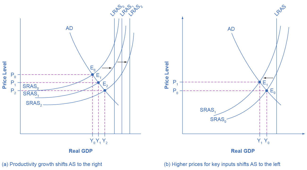

Figure 24.7図 24.7
(a) The rise in productivity causes the SRAS curve to shift to the right. The original equilibrium E0 is at the intersection of AD and SRAS0. When SRAS shifts right, then the new equilibrium E1 is at the intersection of AD and SRAS1, and then yet another equilibrium, E2, is at the intersection of AD and SRAS2. Shifts in SRAS to the right, lead to a greater level of output and to downward pressure on the price level. (b) A higher price for inputs means that at any given price level for outputs, a lower real GDP will be produced so aggregate supply will shift to the left from SRAS0 to SRAS1. The new equilibrium, E1, has a reduced quantity of output and a higher price level than the original equilibrium (E0).
英語のヒント
(a)生産性の上昇によって、SRAS曲線は右へシフトする。元の均衡E0はADとSRAS0の交点にある。SRASが右へシフトすると、新しい均衡E1はADとSRAS1の交点となり、さらに別の均衡E2はADとSRAS2の交点となる。SRASの右方シフトは、生産水準を高め、物価水準に下押し圧力をかける。(b)投入物の価格が上がると、生産物の各物価水準で生産される実質GDPが減るため、総供給はSRAS0からSRAS1へ左にシフトする。新しい均衡E1では、元の均衡E0より生産量が少なく、物価水準が高い。
A shift in the SRAS curve to the right will result in a greater real GDP and downward pressure on the price level, if aggregate demand remains unchanged. However, if this shift in SRAS results from gains in productivity growth, which we typically measure in terms of a few percentage points per year, the effect will be relatively small over a few months or even a couple of years. Recall how in Choice in a World of Scarcity, we said that a nation's production possibilities frontier is fixed in the short run, but shifts out in the long run? This is the same phenomenon using a different model.
英語のヒント
総需要が変わらなければ、SRAS曲線の右方シフトは実質GDPを増やし、物価水準に下押し圧力をかける。しかし、このSRASのシフトが、通常は年数パーセントポイントで測る生産性の向上によるなら、数か月、さらには2年程度の期間では、その効果は比較的小さい。「希少性のある世界での選択」で、一国の生産可能性フロンティアは短期には固定され、長期には外へシフトすると述べたことを思い出そう。これは、別のモデルで表した同じ現象である。
How Changes in Input Prices Shift the AS Curve投入価格の変化はAS曲線をどうシフトさせるか
Higher prices for inputs that are widely used across the entire economy can have a macroeconomic impact on aggregate supply. Examples of such widely used inputs include labor and energy products. Increases in the price of such inputs will cause the SRAS curve to shift to the left, which means that at each given price level for outputs, a higher price for inputs will discourage production because it will reduce the possibilities for earning profits. Figure 24.7 (b) shows the aggregate supply curve shifting to the left, from SRAS0 to SRAS1, causing the equilibrium to move from E0 to E1. The movement from the original equilibrium of E0 to the new equilibrium of E1 will bring a nasty set of effects: reduced GDP or recession, higher unemployment because the economy is now further away from potential GDP, and an inflationary higher price level as well. For example, the U.S. economy experienced recessions in 1974–1975, 1980–1982, 1990–91, 2001, and 2007–2009 that were each preceded or accompanied by a rise in the key input of oil prices. In the 1970s, this pattern of a shift to the left in SRAS leading to a stagnant economy with high unemployment and inflation was nicknamed stagflation.
英語のヒント
経済全体で広く使われる投入物の価格上昇は、総供給にマクロ経済的な影響を与えうる。広く使われる投入物には、労働やエネルギー製品がある。こうした投入物の価格上昇は、SRAS曲線を左へシフトさせる。これは、生産物の各物価水準で、投入物価格の上昇が利益を得る可能性を減らすため、生産を抑えることを意味する。図24.7(b)は、総供給曲線がSRAS0からSRAS1へ左にシフトし、均衡がE0からE1へ移る様子を示す。元の均衡E0から新しい均衡E1への移動は、好ましくない一連の効果をもたらす。GDPの減少または景気後退、潜在GDPからさらに遠ざかることによる失業の増加、そしてインフレを伴う物価水準の上昇である。例えば、米国経済は1974~1975年、1980~1982年、1990~1991年、2001年、2007~2009年に景気後退を経験し、いずれも重要な投入物である石油の価格上昇が先行するか、同時に起きていた。1970年代には、SRASの左方シフトによって高失業とインフレを伴う経済停滞に至るこのパターンに、スタグフレーションという名が付けられた。
Conversely, a decline in the price of a key input like oil will shift the SRAS curve to the right, providing an incentive for more to be produced at every given price level for outputs. From 1985 to 1986, for example, the average price of crude oil fell by almost half, from $24 a barrel to $12 a barrel. Similarly, from 1997 to 1998, the price of a barrel of crude oil dropped from $17 per barrel to $11 per barrel. In both cases, the plummeting oil price led to a situation like that which we presented earlier in Figure 24.7 (a), where the outward shift of SRAS to the right allowed the economy to expand, unemployment to fall, and inflation to decline.
英語のヒント
反対に、石油のような重要な投入物の価格が下がると、SRAS曲線は右へシフトし、生産物の各物価水準でより多く生産する誘因が生まれる。例えば1985~1986年に、原油の平均価格は1バレル24ドルから12ドルへ、ほぼ半減した。同様に1997~1998年には、原油1バレルの価格は17ドルから11ドルへ下がった。どちらの場合も、石油価格の急落は先の図24.7(a)のような状況をもたらした。SRASの右への外方シフトによって、経済は拡大し、失業は減り、インフレは低下できた。
Along with energy prices, two other key inputs that may shift the SRAS curve are the cost of labor, or wages, and the cost of imported goods that we use as inputs for other products. In these cases as well, the lesson is that lower prices for inputs cause SRAS to shift to the right, while higher prices cause it to shift back to the left. Note that, unlike changes in productivity, changes in input prices do not generally cause LRAS to shift, only SRAS.
英語のヒント
エネルギー価格と並んで、SRAS曲線をシフトさせうる重要な投入物には、労働費用、すなわち賃金と、他の製品の投入物として使う輸入品の費用がある。これらの場合も、投入物の価格低下はSRASを右へ、価格上昇は左へシフトさせるというのが教訓である。生産性の変化と違い、投入価格の変化は通常LRASをシフトさせず、SRASだけをシフトさせることに注意しよう。