Equilibrium in the Aggregate Demand/Aggregate Supply Model総需要・総供給モデルの均衡
The intersection of the aggregate supply and aggregate demand curves shows the equilibrium level of real GDP and the equilibrium price level in the economy. At a relatively low price level for output, firms have little incentive to produce, although consumers would be willing to purchase a large quantity of output. As the price level rises, aggregate supply rises and aggregate demand falls until the equilibrium point is reached.
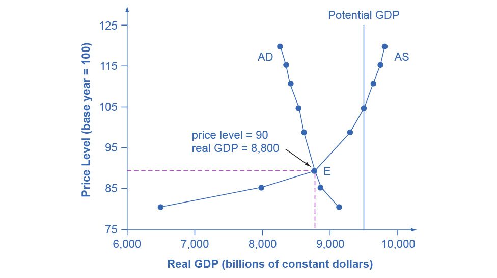
Figure 24.6 combines the AS curve from Figure 24.3 and the AD curve from Figure 24.4 and places them both on a single diagram. In this example, the equilibrium point occurs at point E, at a price level of 90 and an output level of 8,800.
Copyright Rice University, OpenStax, under CC-BY 4.0 license. · CC BY 4.0 · Source出典
Figure 24.6図 24.6
The equilibrium, where aggregate supply (AS) equals aggregate demand (AD), occurs at a price level of 90 and an output level of 8,800.
英語のヒント
総供給(AS)と総需要(AD)が等しくなる均衡は、物価水準90、生産水準8800で生じる。
Confusion sometimes arises between the aggregate supply and aggregate demand model and the microeconomic analysis of demand and supply in particular markets for goods, services, labor, and capital. Read the following Clear It Up feature to gain an understanding of whether AS and AD are macro or micro.
In the Clear It Up feature titled “Why does AS cross potential GDP?” we differentiated between short run changes in aggregate supply which the AS curve shows and long run changes in aggregate supply which the vertical line at potential GDP defines. In the short run, if demand is too low (or too high), it is possible for producers to supply less GDP (or more GDP) than potential. In the long run, however, producers are limited to producing at potential GDP. For this reason, we may also refer to what we have been calling the AS curve as the short run aggregate supply (SRAS) curve. We may also refer to the vertical line at potential GDP as the long run aggregate supply (LRAS) curve.