第7章生産・費用・産業構造
Economies of Scale規模の経済
Once a firm has determined the least costly production technology, it can consider the optimal scale of production, or quantity of output to produce. Many industries experience economies of scale. Economies of scale refers to the situation where, as the quantity of output goes up, the cost per unit goes down. This is the idea behind “warehouse stores” like Costco or Walmart. In everyday language: a larger factory can produce at a lower average cost than a smaller factory.
英語のヒント
最も安い生産技術を決めたら、最適な生産規模、すなわち生産量を考えられる。多くの産業には規模の経済がある。これは、産出量が増えると単位当たり費用が下がる状態だ。コストコやウォルマートのような「倉庫型店舗」の背後にある考えでもある。日常的な言い方なら、大きな工場は小さな工場より低い平均費用で生産できる、ということだ。
Figure 7.9 illustrates the idea of economies of scale, showing the average cost of producing an alarm clock falling as the quantity of output rises. For a small-sized factory like S, with an output level of 1,000, the average cost of production is $12 per alarm clock. For a medium-sized factory like M, with an output level of 2,000, the average cost of production falls to $8 per alarm clock. For a large factory like L, with an output of 5,000, the average cost of production declines still further to $4 per alarm clock.
英語のヒント
図7.9は、目覚まし時計の生産量が増えると平均費用が下がる様子で、規模の経済を示す。Sのような小工場は1,000個を生産し、1個当たり平均費用は12ドルだ。Mのような中規模工場は2,000個を生産し、平均費用は8ドルへ下がる。Lのような大工場では5,000個を生産し、平均費用はさらに4ドルへ下がる。
Economies of Scale規模の経済
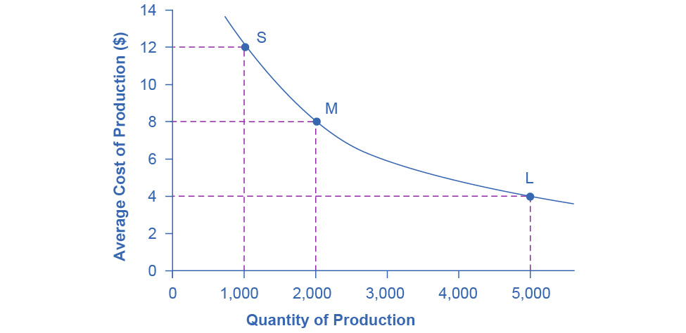
Figure 7.9図 7.9
A small factory like S produces 1,000 alarm clocks at an average cost of $12 per clock. A medium factory like M produces 2,000 alarm clocks at a cost of $8 per clock. A large factory like L produces 5,000 alarm clocks at a cost of $4 per clock. Economies of scale exist when the larger scale of production leads to lower average costs.
英語のヒント
小工場Sは目覚まし時計1,000個を1個当たり平均12ドル、中規模工場Mは2,000個を8ドル、大工場Lは5,000個を4ドルで生産する。生産規模の拡大が平均費用の低下につながるとき、規模の経済がある。
The average cost curve in Figure 7.9 may appear similar to the average cost curves we presented earlier in this chapter, although it is downward-sloping rather than U-shaped. However, there is one major difference. The economies of scale curve is a long-run average cost curve, because it allows all factors of production to change. The short-run average cost curves we presented earlier in this chapter assumed the existence of fixed costs, and only variable costs were allowed to change.
英語のヒント
図7.9の平均費用曲線は、U字形ではなく右下がりだが、前に示した平均費用曲線に似て見えるかもしれない。しかし、大きな違いがある。規模の経済の曲線は、すべての生産要素を変えられる長期平均費用曲線である。前に示した短期平均費用曲線では固定費用の存在を仮定し、変えられるのは可変費用だけだった。
One prominent example of economies of scale occurs in the chemical industry. Chemical plants have many pipes. The cost of the materials for producing a pipe is related to the circumference of the pipe and its length. However, the cross-section area of the pipe determines the volume of chemicals that can flow through it. The calculations in Table 7.16 show that a pipe which uses twice as much material to make (as shown by the circumference) can actually carry four times the volume of chemicals because the pipe's cross-section area rises by a factor of four (as the Area column below shows).
英語のヒント
規模の経済の顕著な例が化学産業だ。化学工場には多数の配管がある。管を作る材料費は管の円周と長さに関係するが、流せる化学物質の量を決めるのは断面積である。表7.16の計算は、円周で示す材料の量を2倍にして作った管が、実際には4倍の化学物質を流せることを示す。面積の列のように、断面積が4倍になるためだ。
Circumference () 円周() |
Area () 面積() |
|
|---|---|---|
4-inch pipe 4インチ管 |
12.5 inches 12.5インチ |
12.5 square inches 12.5平方インチ |
8-inch pipe 8インチ管 |
25.1 inches 25.1インチ |
50.2 square inches 50.2平方インチ |
16-inch pipe 16インチ管 |
50.2 inches 50.2インチ |
201.1 square inches 201.1平方インチ |
A doubling of the cost of producing the pipe allows the chemical firm to process four times as much material. This pattern is a major reason for economies of scale in chemical production, which uses a large quantity of pipes. Of course, economies of scale in a chemical plant are more complex than this simple calculation suggests. However, the chemical engineers who design these plants have long used what they call the “six-tenths rule,” a rule of thumb which holds that increasing the quantity produced in a chemical plant by a certain percentage will increase total cost by only six-tenths as much.
英語のヒント
管の製作費用を2倍にすると、化学企業は4倍の物質を処理できる。大量の配管を使う化学生産で規模の経済が生じる大きな理由だ。実際の化学工場の規模の経済は、この単純な計算より複雑である。しかし、設計する化学技術者は長く「6割則」という経験則を使ってきた。工場の生産量を一定の割合だけ増やしても、総費用はその6割の割合しか増えないというものだ。
Shapes of Long-Run Average Cost Curves長期平均費用曲線の形
While in the short run firms are limited to operating on a single average cost curve (corresponding to the level of fixed costs they have chosen), in the long run when all costs are variable, they can choose to operate on any average cost curve. Thus, the long-run average cost (LRAC) curve is actually based on a group of short-run average cost (SRAC) curves, each of which represents one specific level of fixed costs. More precisely, the long-run average cost curve will be the least expensive average cost curve for any level of output. Figure 7.10 shows how we build the long-run average cost curve from a group of short-run average cost curves. Five short-run-average cost curves appear on the diagram. Each SRAC curve represents a different level of fixed costs. For example, you can imagine SRAC1 as a small factory, SRAC2 as a medium factory, SRAC3 as a large factory, and SRAC4 and SRAC5 as very large and ultra-large. Although this diagram shows only five SRAC curves, presumably there are an infinite number of other SRAC curves between the ones that we show. Think of this family of short-run average cost curves as representing different choices for a firm that is planning its level of investment in fixed cost physical capital—knowing that different choices about capital investment in the present will cause it to end up with different short-run average cost curves in the future.
英語のヒント
短期には、企業は選んだ固定費用の水準に対応する一つの平均費用曲線上でしか操業できない。すべての費用が可変になる長期には、どの平均費用曲線で操業するか選べる。そのため長期平均費用LRAC曲線は、異なる固定費用の水準を表す短期平均費用SRAC曲線の集まりに基づく。より正確には、各産出量で最も安い平均費用を示す曲線だ。図7.10は、短期平均費用曲線の集まりから長期平均費用曲線を作る方法を示す。5本のSRAC曲線は、それぞれ異なる固定費用を表す。例えばSRAC1を小工場、SRAC2を中規模、SRAC3を大規模、SRAC4とSRAC5を非常に大きい工場と超大型工場と考えられる。図には5本しかないが、その間には無数の別のSRAC曲線があると考えられる。この曲線群は、固定費用となる物的資本への投資を計画する企業の選択肢を表す。今の資本投資の選択によって、将来の短期平均費用曲線が変わるのである。
From Short-Run Average Cost Curves to Long-Run Average Cost Curves短期平均費用曲線から長期平均費用曲線へ
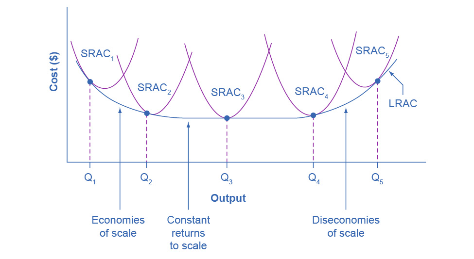


Figure 7.10図 7.10
The five different short-run average cost (SRAC) curves each represents a different level of fixed costs, from the low level of fixed costs at SRAC1 to the high level of fixed costs at SRAC5. Other SRAC curves, not in the diagram, lie between the ones that are here. The long-run average cost (LRAC) curve shows the lowest cost for producing each quantity of output when fixed costs can vary, and so it is formed by the bottom edge of the family of SRAC curves. If a firm wished to produce quantity Q3, it would choose the fixed costs associated with SRAC3.
英語のヒント
5本の短期平均費用SRAC曲線は、SRAC1の低い固定費用からSRAC5の高い固定費用まで、異なる水準を表す。描かれていないSRAC曲線が、その間にもある。長期平均費用LRAC曲線は、固定費用を変えられるときの各産出量の最小費用を示すため、SRAC曲線群の下側の縁になる。Q3を生産したい企業は、SRAC3に対応する固定費用を選ぶ。
The long-run average cost curve shows the cost of producing each quantity in the long run, when the firm can choose its level of fixed costs and thus choose which short-run average costs it desires. If the firm plans to produce in the long run at an output of Q3, it should make the set of investments that will lead it to locate on SRAC3, which allows producing q3 at the lowest cost. A firm that intends to produce Q3 would be foolish to choose the level of fixed costs at SRAC2 or SRAC4. At SRAC2 the level of fixed costs is too low for producing Q3 at lowest possible cost, and producing q3 would require adding a very high level of variable costs and make the average cost very high. At SRAC4, the level of fixed costs is too high for producing q3 at lowest possible cost, and again average costs would be very high as a result.
英語のヒント
長期平均費用曲線は、企業が固定費用の水準、したがって希望する短期平均費用を選べる長期に、各数量を生産する費用を示す。長期にQ3を生産する計画なら、SRAC3上に位置するよう投資すべきだ。q3を最も安く生産できるからである。Q3を生産したいのに、SRAC2やSRAC4の固定費用を選ぶのは賢明ではない。SRAC2では、Q3を最安で生産するには固定費用が低すぎる。q3を生産するために可変費用を大幅に増やす必要があり、平均費用が非常に高くなる。SRAC4では、q3を最安で生産するには固定費用が高すぎ、やはり平均費用が非常に高くなる。
The shape of the long-run cost curve, in Figure 7.10, is fairly common for many industries. The left-hand portion of the long-run average cost curve, where it is downward- sloping from output levels Q1 to Q2 to Q3, illustrates the case of economies of scale. In this portion of the long-run average cost curve, larger scale leads to lower average costs. We illustrated this pattern earlier in Figure 7.9.
英語のヒント
In the middle portion of the long-run average cost curve, the flat portion of the curve around Q3, economies of scale have been exhausted. In this situation, allowing all inputs to expand does not much change the average cost of production. We call this constant returns to scale. In this LRAC curve range, the average cost of production does not change much as scale rises or falls. The following Clear It Up feature explains where diminishing marginal returns fit into this analysis.
英語のヒント
長期平均費用曲線の中央、Q3付近の平らな部分では、規模の経済を使い尽くしている。すべての投入物を増やしても、平均生産費用はあまり変わらない。これを規模に関する収穫一定という。この範囲では、規模が増減しても平均費用はあまり変わらない。次の「疑問を解く」では、限界収穫逓減をこの分析にどう位置付けるか説明する。
Finally, the right-hand portion of the long-run average cost curve, running from output level Q4 to Q5, shows a situation where, as the level of output and the scale rises, average costs rise as well. We call this situation diseconomies of scale. A firm or a factory can grow so large that it becomes very difficult to manage, resulting in unnecessarily high costs as many layers of management try to communicate with workers and with each other, and as failures to communicate lead to disruptions in the flow of work and materials. Not many overly large factories exist in the real world, because with their very high production costs, they are unable to compete for long against plants with lower average costs of production. However, in some planned economies, like the economy of the old Soviet Union, plants that were so large as to be grossly inefficient were able to continue operating for a long time because government economic planners protected them from competition and ensured that they would not make losses.
英語のヒント
最後に、長期平均費用曲線の右側、Q4からQ5の部分は、産出量と規模が増すと平均費用も上がる状況を示す。これを規模の不経済という。企業や工場が大きくなりすぎると管理が難しくなる。幾層もの管理部門が従業員やほかの部門と連絡し、伝達の失敗が仕事や資材の流れを乱すため、不必要に費用が高くなる。現実に過大な工場があまりないのは、高い生産費用では、低い平均費用の工場と長く競争できないためだ。しかし旧ソ連などの計画経済では、政府の経済計画担当者が競争から保護し、損失が出ないようにしたため、大きすぎて著しく非効率な工場も長く操業できた。
Diseconomies of scale can also be present across an entire firm, not just a large factory. The leviathan effect can hit firms that become too large to run efficiently, across the entirety of the enterprise. Firms that shrink their operations are often responding to finding itself in the diseconomies region, thus moving back to a lower average cost at a lower output level.
英語のヒント
規模の不経済は大工場だけでなく、企業全体でも生じる。効率よく運営できないほど大きくなった企業には、事業全体に巨大化の弊害が及ぶ。事業を縮小する企業は、規模の不経済の範囲に入ったことへの対応として、低い産出量で低い平均費用へ戻ろうとしている場合が多い。