付録

Linear Regression線形回帰

Sample Data標本データ

The following data is real. The percent of declared ethnic minority students at De Anza College for selected years from 1970–1995 was:

英語のヒント

次のデータは実際のデータである。1970～1995年のうち選ばれた年について、デアンザ・カレッジで民族的少数派であると申告した学生の割合は、次のとおりだった。

Table G.2表 G.2
The independent variable is "Year," while the independent variable is "Student Ethnic Minority Percent."
独立変数は「年」であり、もう一方の独立変数は「民族的少数派の学生の割合」である。
Year 年	Student Ethnic Minority Percentage 民族的少数派の学生の割合（%）
1970	14.13
1973	12.27
1976	14.08
1979	18.16
1982	27.64
1983	28.72
1986	31.86
1989	33.14
1992	45.37
1995	53.1

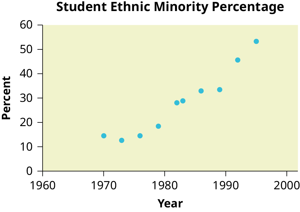
与えられたデータの散布図。横軸は年、縦軸は百分率を表す。各点は、強い曲線的な上昇傾向を示す。 — Figure G.1図 G.1
By hand, verify the scatterplot above.
手作業で上の散布図を確認せよ。

To enter data and do linear regression:データを入力し、線形回帰を行う

ON Turns calculator on.
ONで電卓の電源を入れる。

Copyright Rice University, OpenStax, Introductory Statistics 2e, CC BY 4.0. · CC BY 4.0 · Source出典
Before accessing this program, be sure to turn off all plots.
このプログラムを開く前に、必ずすべてのグラフを無効にする。
- Access graphing mode.
  グラフ作成モードを開く。
  
  Copyright Rice University, OpenStax, Introductory Statistics 2e, CC BY 4.0. · CC BY 4.0 · Source出典
  
  , [STAT PLOT]
  、[STAT PLOT]
- Turn off all plots.
  すべてのグラフを無効にする。
  
  Copyright Rice University, OpenStax, Introductory Statistics 2e, CC BY 4.0. · CC BY 4.0 · Source出典
  
  ,
  
  Copyright Rice University, OpenStax, Introductory Statistics 2e, CC BY 4.0. · CC BY 4.0 · Source出典
Round to three decimal places. To do so:
小数第3位に丸める。手順は次のとおり。
- Access the mode menu.
  MODEメニューを開く。
  
  Copyright Rice University, OpenStax, Introductory Statistics 2e, CC BY 4.0. · CC BY 4.0 · Source出典
  
  , [STAT PLOT]
  、[STAT PLOT]
- Navigate to <Float> and then to the right to <3>.
  <Float>へ移動し、続いて右側の<3>へ移動する。
  
  Copyright Rice University, OpenStax, Introductory Statistics 2e, CC BY 4.0. · CC BY 4.0 · Source出典
  
  Copyright Rice University, OpenStax, Introductory Statistics 2e, CC BY 4.0. · CC BY 4.0 · Source出典
- All numbers will be rounded to three decimal places until changed.
  設定を変更するまで、すべての数値が小数第3位に丸められる。
  
  Copyright Rice University, OpenStax, Introductory Statistics 2e, CC BY 4.0. · CC BY 4.0 · Source出典
Enter statistics mode and clear lists [L1] and [L2], as describe previously.
統計モードを開き、前述の方法でリスト[L1]と[L2]を消去する。

Copyright Rice University, OpenStax, Introductory Statistics 2e, CC BY 4.0. · CC BY 4.0 · Source出典

,

Copyright Rice University, OpenStax, Introductory Statistics 2e, CC BY 4.0. · CC BY 4.0 · Source出典
Enter editing mode to insert values for x and y.
編集モードを開き、xとyの値を入力する。

Copyright Rice University, OpenStax, Introductory Statistics 2e, CC BY 4.0. · CC BY 4.0 · Source出典

,

Copyright Rice University, OpenStax, Introductory Statistics 2e, CC BY 4.0. · CC BY 4.0 · Source出典
Enter each value. Press
各値を入力する。次のキーを押す。

Copyright Rice University, OpenStax, Introductory Statistics 2e, CC BY 4.0. · CC BY 4.0 · Source出典

to continue.
これで次へ進む。

To display the correlation coefficient:相関係数を表示する

Access the catalog.
カタログを開く。

Copyright Rice University, OpenStax, Introductory Statistics 2e, CC BY 4.0. · CC BY 4.0 · Source出典

, [CATALOG]
、[CATALOG]
Arrow down and select <DiagnosticOn>
下向き矢印キーで移動し、<DiagnosticOn>を選択する。

Copyright Rice University, OpenStax, Introductory Statistics 2e, CC BY 4.0. · CC BY 4.0 · Source出典

... ,

Copyright Rice University, OpenStax, Introductory Statistics 2e, CC BY 4.0. · CC BY 4.0 · Source出典

,

Copyright Rice University, OpenStax, Introductory Statistics 2e, CC BY 4.0. · CC BY 4.0 · Source出典
$r$ and $r^{2}$ will be displayed during regression calculations.
回帰計算の際に、 $r$ と $r^{2}$ が表示される。
Access linear regression.
線形回帰を開く。

Copyright Rice University, OpenStax, Introductory Statistics 2e, CC BY 4.0. · CC BY 4.0 · Source出典

Copyright Rice University, OpenStax, Introductory Statistics 2e, CC BY 4.0. · CC BY 4.0 · Source出典
Select the form of y = a + bx.
y = a + bxの形式を選択する。

Copyright Rice University, OpenStax, Introductory Statistics 2e, CC BY 4.0. · CC BY 4.0 · Source出典

,

Copyright Rice University, OpenStax, Introductory Statistics 2e, CC BY 4.0. · CC BY 4.0 · Source出典

The display will show:

画面には次のように表示される。

LinRegLinReg

y = a + bx
a = –3176.909
a = −3176.909
b = 1.617
r = 2 0.924
r = 0.961

This means the Line of Best Fit (Least Squares Line) is:

これは、最適直線（最小二乗直線）が次のとおりであることを意味する。

y = –3176.909 + 1.617x
y = −3176.909 + 1.617x
Percent = –3176.909 + 1.617 (year #)
割合（%）= −3176.909 + 1.617 × 年の数値

The correlation coefficient r = 0.961

相関係数はr = 0.961である。

To see the scatter plot:散布図を表示する

Access graphing mode.
グラフ作成モードを開く。

Copyright Rice University, OpenStax, Introductory Statistics 2e, CC BY 4.0. · CC BY 4.0 · Source出典

, [STAT PLOT]
、[STAT PLOT]
Select <1:plot 1> To access plotting - first graph.
<1:plot 1>を選択し、1つ目のグラフの設定を開く。

Copyright Rice University, OpenStax, Introductory Statistics 2e, CC BY 4.0. · CC BY 4.0 · Source出典
Navigate and select <ON> to turn on Plot 1.
<ON>
<ON>に移動して選択し、Plot 1を有効にする。<ON>

Copyright Rice University, OpenStax, Introductory Statistics 2e, CC BY 4.0. · CC BY 4.0 · Source出典
Navigate to the first picture.
最初の図へ移動する。
Select the scatter plot.
散布図を選択する。

Copyright Rice University, OpenStax, Introductory Statistics 2e, CC BY 4.0. · CC BY 4.0 · Source出典
Navigate to <Xlist>.
<Xlist>へ移動する。
If [L1] is not selected, press
[L1]が選択されていなければ、次のキーを押す。

Copyright Rice University, OpenStax, Introductory Statistics 2e, CC BY 4.0. · CC BY 4.0 · Source出典

, [L1] to select it.
続いて[L1]を押して選択する。
Confirm that the data values are in [L1].
<ON>
データの値が[L1]にあることを確認する。<ON>

Copyright Rice University, OpenStax, Introductory Statistics 2e, CC BY 4.0. · CC BY 4.0 · Source出典
Navigate to <Ylist>.
<Ylist>へ移動する。
Select that the frequencies are in [L2].
度数のリストとして[L2]を選択する。

Copyright Rice University, OpenStax, Introductory Statistics 2e, CC BY 4.0. · CC BY 4.0 · Source出典

, [L2] ,
、[L2]、

Copyright Rice University, OpenStax, Introductory Statistics 2e, CC BY 4.0. · CC BY 4.0 · Source出典
Go back to access other graphs.
前に戻り、ほかのグラフを開く。

Copyright Rice University, OpenStax, Introductory Statistics 2e, CC BY 4.0. · CC BY 4.0 · Source出典

, [STAT PLOT]
、[STAT PLOT]
Use the arrows to turn off the remaining plots.
矢印キーを使い、残りのグラフを無効にする。
Access window mode to set the graph parameters.
WINDOWモードを開き、グラフの設定値を入力する。

Copyright Rice University, OpenStax, Introductory Statistics 2e, CC BY 4.0. · CC BY 4.0 · Source出典
- $X_{\min} = 1970$
- $X_{\max} = 2000$
- $X_{s c l} = 10$ (spacing of tick marks on x-axis)
  $X_{s c l} = 10$ （x軸の目盛りの間隔）
- $Y_{\min} = - 0.05$
- $Y_{\max} = 60$
- $Y_{s c l} = 10$ (spacing of tick marks on y-axis)
  $Y_{s c l} = 10$ （y軸の目盛りの間隔）
- $X_{r e s} = 1$
Be sure to deselect or clear all equations before graphing, using the instructions above.
グラフを描く前に、前述の手順で、必ずすべての式の選択を解除するか、式を消去する。
Press the graph button to see the scatter plot.
GRAPHキーを押し、散布図を表示する。

Copyright Rice University, OpenStax, Introductory Statistics 2e, CC BY 4.0. · CC BY 4.0 · Source出典

To see the regression graph:回帰直線のグラフを表示する

Access the equation menu. The regression equation will be put into Y1.
式のメニューを開く。回帰式をY1へ入力する。

Copyright Rice University, OpenStax, Introductory Statistics 2e, CC BY 4.0. · CC BY 4.0 · Source出典
Access the vars menu and navigate to <5: Statistics>.
VARSメニューを開き、<5: Statistics>へ移動する。

Copyright Rice University, OpenStax, Introductory Statistics 2e, CC BY 4.0. · CC BY 4.0 · Source出典

,

Copyright Rice University, OpenStax, Introductory Statistics 2e, CC BY 4.0. · CC BY 4.0 · Source出典
Navigate to <EQ>.
<EQ>へ移動する。
<1: RegEQ> contains the regression equation which will be entered in Y1.
<1: RegEQ>には、Y1へ入力する回帰式が入っている。

Copyright Rice University, OpenStax, Introductory Statistics 2e, CC BY 4.0. · CC BY 4.0 · Source出典
Press the graphing mode button. The regression line will be superimposed over the scatter plot.
英語のヒント
グラフ表示モードのキーを押す。回帰直線が散布図に重ねて表示される。

Copyright Rice University, OpenStax, Introductory Statistics 2e, CC BY 4.0. · CC BY 4.0 · Source出典

To see the residuals and use them to calculate the critical point for an outlier:残差を表示し、外れ値判定の臨界値を計算する

Access the list. RESID will be an item on the menu. Navigate to it.
リストを開く。メニューにRESIDという項目があるので、そこへ移動する。

Copyright Rice University, OpenStax, Introductory Statistics 2e, CC BY 4.0. · CC BY 4.0 · Source出典

, [LIST], <RESID>
、[LIST]、<RESID>
Confirm twice to view the list of residuals. Use the arrows to select them.
2回確定して残差のリストを表示する。矢印キーで各残差を選択する。

Copyright Rice University, OpenStax, Introductory Statistics 2e, CC BY 4.0. · CC BY 4.0 · Source出典

,

Copyright Rice University, OpenStax, Introductory Statistics 2e, CC BY 4.0. · CC BY 4.0 · Source出典
The critical point for an outlier is: $1.9 V \frac{SSE}{n - 2}$ where:
外れ値判定の臨界値は $1.9 V \frac{SSE}{n - 2}$ である。各記号の意味は次のとおり。
- $n$ = number of pairs of data
  $n$ = データのペア数
- $SSE$ = sum of the squared errors
  $SSE$ = 誤差平方和
- $Σ {residual}^{2}$
Store the residuals in [L3].
残差を[L3]に保存する。

Copyright Rice University, OpenStax, Introductory Statistics 2e, CC BY 4.0. · CC BY 4.0 · Source出典

,

Copyright Rice University, OpenStax, Introductory Statistics 2e, CC BY 4.0. · CC BY 4.0 · Source出典

, [L3] ,
、[L3]、

Copyright Rice University, OpenStax, Introductory Statistics 2e, CC BY 4.0. · CC BY 4.0 · Source出典
Calculate the $\frac{{Σresidual}^{2}}{n - 2}$ . Note that $n - 2 = 8$
$\frac{{Σresidual}^{2}}{n - 2}$ を計算する。 $n - 2 = 8$ であることに注意する。

Copyright Rice University, OpenStax, Introductory Statistics 2e, CC BY 4.0. · CC BY 4.0 · Source出典

, [L3] ,
、[L3]、

Copyright Rice University, OpenStax, Introductory Statistics 2e, CC BY 4.0. · CC BY 4.0 · Source出典

,

Copyright Rice University, OpenStax, Introductory Statistics 2e, CC BY 4.0. · CC BY 4.0 · Source出典

,

Copyright Rice University, OpenStax, Introductory Statistics 2e, CC BY 4.0. · CC BY 4.0 · Source出典
Store this value in [L4].
この値を[L4]に保存する。

Copyright Rice University, OpenStax, Introductory Statistics 2e, CC BY 4.0. · CC BY 4.0 · Source出典

,

Copyright Rice University, OpenStax, Introductory Statistics 2e, CC BY 4.0. · CC BY 4.0 · Source出典

, [L4] ,
、[L4]、

Copyright Rice University, OpenStax, Introductory Statistics 2e, CC BY 4.0. · CC BY 4.0 · Source出典
Calculate the critical value using the equation above.
上の式を使って臨界値を計算する。

Copyright Rice University, OpenStax, Introductory Statistics 2e, CC BY 4.0. · CC BY 4.0 · Source出典

,

Copyright Rice University, OpenStax, Introductory Statistics 2e, CC BY 4.0. · CC BY 4.0 · Source出典

,

Copyright Rice University, OpenStax, Introductory Statistics 2e, CC BY 4.0. · CC BY 4.0 · Source出典

,

Copyright Rice University, OpenStax, Introductory Statistics 2e, CC BY 4.0. · CC BY 4.0 · Source出典

,

Copyright Rice University, OpenStax, Introductory Statistics 2e, CC BY 4.0. · CC BY 4.0 · Source出典

, [V] ,
、[V]、

Copyright Rice University, OpenStax, Introductory Statistics 2e, CC BY 4.0. · CC BY 4.0 · Source出典

, [LIST]
、[LIST]

Copyright Rice University, OpenStax, Introductory Statistics 2e, CC BY 4.0. · CC BY 4.0 · Source出典

,

Copyright Rice University, OpenStax, Introductory Statistics 2e, CC BY 4.0. · CC BY 4.0 · Source出典

,

Copyright Rice University, OpenStax, Introductory Statistics 2e, CC BY 4.0. · CC BY 4.0 · Source出典

,

Copyright Rice University, OpenStax, Introductory Statistics 2e, CC BY 4.0. · CC BY 4.0 · Source出典

, [L4] ,
、[L4]、

Copyright Rice University, OpenStax, Introductory Statistics 2e, CC BY 4.0. · CC BY 4.0 · Source出典

,

Copyright Rice University, OpenStax, Introductory Statistics 2e, CC BY 4.0. · CC BY 4.0 · Source出典

,

Copyright Rice University, OpenStax, Introductory Statistics 2e, CC BY 4.0. · CC BY 4.0 · Source出典
Verify that the calculator displays: 7.642669563. This is the critical value.
電卓に7.642669563と表示されることを確認する。これが臨界値である。
Compare the absolute value of each residual value in [L3] to 7.64. If the absolute value is greater than 7.64, then the (x, y) corresponding point is an outlier. In this case, none of the points is an outlier.
英語のヒント
[L3]の各残差の絶対値を7.64と比較する。絶対値が7.64より大きければ、対応する点(x, y)は外れ値である。この例では、外れ値となる点はない。

To obtain estimates of y for various x-values:さまざまなxの値に対するyの推定値を求める

There are various ways to determine estimates for "y." One way is to substitute values for "x" in the equation. Another way is to use the

「y」の推定値を求める方法はいくつかある。1つは、式の「x」に値を代入する方法である。もう1つは、次のキーを使う方法である。

on the graph of the regression line.

回帰直線のグラフ上でこのキーを使う。