第5章連続確率変数

Introductionはじめに

さまざまな高さのダイコンが土から芽を出している画像。 — Figure 5.1図 5.1
The heights of these radish plants are continuous random variables. (credit: modification of work “Radish (Raphanus sativus): White rust caused by Albugo candida” by Scot Nelson/ Flickr, Public Domain)
これらのダイコンの草丈は連続確率変数である。（出典：Scot Nelson / Flickrによる「ダイコン（Raphanus sativus）：Albugo candidaによる白さび病」を改変、パブリックドメイン）

Continuous random variables have many applications. Baseball batting averages, IQ scores, the length of time a long distance telephone call lasts, the amount of money a person carries, the length of time a computer chip lasts, and SAT scores are just a few. The field of reliability depends on a variety of continuous random variables.

英語のヒント

連続確率変数には多くの応用がある。野球の打率、IQスコア、長距離電話の通話時間、所持金の額、コンピューターチップの寿命、SATの得点は、そのごく一部である。信頼性の分野では、さまざまな連続確率変数を用いる。

NOTE注意

The values of discrete and continuous random variables can be ambiguous. For example, if X is equal to the number of miles (to the nearest mile) you drive to work, then X is a discrete random variable. You count the miles. If X is the distance you drive to work, then you measure values of X and X is a continuous random variable. For a second example, if X is equal to the number of books in a backpack, then X is a discrete random variable. If X is the weight of a book, then X is a continuous random variable because weights are measured. How the random variable is defined is very important.

英語のヒント

離散確率変数と連続確率変数の値の区別は、曖昧になることがある。たとえば、Xを車で通勤する距離のマイル数（1マイル単位に丸める）とすれば、Xは離散確率変数である。マイル数を数えるからである。Xを車で通勤する距離とすれば、Xの値を測定するので、Xは連続確率変数になる。別の例として、Xがリュック内の本の冊数なら、Xは離散確率変数である。Xが本の重さなら、重さを測定するため、連続確率変数となる。確率変数をどのように定義するかは非常に重要である。

Properties of Continuous Probability Distributions連続確率分布の性質

The graph of a continuous probability distribution is a curve. Probability is represented by area under the curve.

連続確率分布のグラフは曲線である。確率は曲線の下の面積で表される。

The curve is called the probability density function (abbreviated as pdf). We use the symbol f(x) to represent the curve. f(x) is the function that corresponds to the graph; we use the density function f(x) to draw the graph of the probability distribution.

英語のヒント

この曲線を確率密度関数（略してpdf）と呼ぶ。曲線を記号f(x)で表す。f(x)はグラフに対応する関数であり、密度関数f(x)を使って確率分布のグラフを描く。

Area under the curve is given by a different function called the cumulative distribution function (abbreviated as cdf). The cumulative distribution function is used to evaluate probability as area.

英語のヒント

曲線の下の面積は、累積分布関数（略してcdf）という別の関数によって与えられる。累積分布関数を使い、確率を面積として求める。

The outcomes are measured, not counted.
結果は数えるのではなく、測定する。
The entire area under the curve and above the x-axis is equal to one.
曲線より下、x軸より上にある全体の面積は1である。
Probability is found for intervals of x values rather than for individual x values.
個々のxの値ではなく、xの値の区間について確率を求める。
P(c < x < d) is the probability that the random variable X is in the interval between the values c and d. P(c < x < d) is the area under the curve, above the x-axis, to the right of c and the left of d.
P(c < x < d)は、確率変数Xがcとdの間の区間にある確率である。P(c < x < d)は、曲線より下、x軸より上、cより右、dより左の面積である。
P(x = c) = 0 The probability that x takes on any single individual value is zero. The area below the curve, above the x-axis, and between x = c and x = c has no width, and therefore no area (area = 0). Since the probability is equal to the area, the probability is also zero.
P(x = c) = 0。xがある特定の一つの値を取る確率は0である。曲線より下、x軸より上で、x = cとx = cの間の領域には幅がないため、面積もない（面積 = 0）。確率は面積に等しいので、確率も0になる。
P(c < x < d) is the same as P(c ≤ x ≤ d) because probability is equal to area.
確率は面積に等しいので、P(c < x < d)とP(c ≤ x ≤ d)は同じである。

We will find the area that represents probability by using geometry, formulas, technology, or probability tables. In general, calculus is needed to find the area under the curve for many probability density functions. When we use formulas to find the area in this textbook, the formulas were found by using the techniques of integral calculus. However, because most students taking this course have not studied calculus, we will not be using calculus in this textbook.

英語のヒント

幾何、公式、機器、確率表を使って、確率を表す面積を求めていく。一般に、多くの確率密度関数で曲線の下の面積を求めるには微積分が必要である。本書で面積を求める際に使う公式は、積分の手法で導かれたものである。ただし、この科目を履修する学生の多くは微積分を学んでいないため、本書では微積分を使わない。

There are many continuous probability distributions. When using a continuous probability distribution to model probability, the distribution used is selected to model and fit the particular situation in the best way.

連続確率分布には多くの種類がある。連続確率分布を確率のモデルとして使うときは、個々の状況を最もうまく表現し、適合する分布を選ぶ。

In this chapter and the next, we will study the uniform distribution, the exponential distribution, and the normal distribution. The following graphs illustrate these distributions.

本章と次章では、一様分布、指数分布、正規分布を学ぶ。次のグラフは、これらの分布を示している。

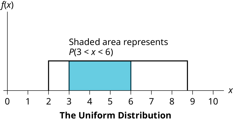
一様分布のグラフ。横軸は0から10で、分布はx = 2からx = 8.8までの長方形で表される。長方形内のx = 3からx = 6までが着色され、P(3 x < 6)を表している。 — Figure 5.2図 5.2
The graph shows a Uniform Distribution with the area between x = 3 and x = 6 shaded to represent the probability that the value of the random variable X is in the interval between three and six.
一様分布のグラフ。x = 3とx = 6の間を着色し、確率変数Xの値が3と6の間の区間にある確率を表している。

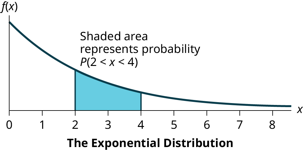
指数分布のグラフ。曲線はy軸上の点から右下がりに伸び、右端に向かってx軸に近づく。曲線の下のx = 2からx = 4までが着色され、P(2 < x < 4)を表している。 — Figure 5.3図 5.3
The graph shows an Exponential Distribution with the area between x = 2 and x = 4 shaded to represent the probability that the value of the random variable X is in the interval between two and four.
指数分布のグラフ。x = 2とx = 4の間を着色し、確率変数Xの値が2と4の間の区間にある確率を表している。

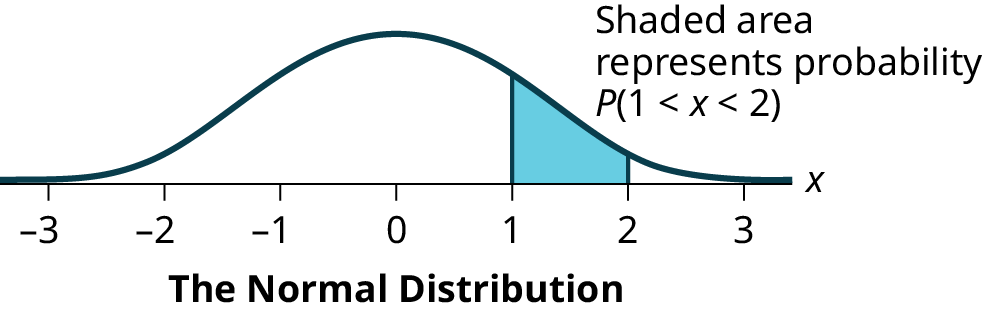
横軸に−3から3まで1刻みの目盛りがある正規分布曲線。頂点は横軸の0に対応する。1と2から曲線へ縦線が伸び、その間が着色されている。「着色部分は確率P(1 < x < 2)を表す」と記されている。 — Figure 5.4図 5.4
The graph shows the Standard Normal Distribution with the area between x = 1 and x = 2 shaded to represent the probability that the value of the random variable X is in the interval between one and two.
標準正規分布のグラフ。x = 1とx = 2の間を着色し、確率変数Xの値が1と2の間の区間にある確率を表している。

Uniform Distribution

一様分布

a continuous random variable (RV) that has equally likely outcomes over the domain, a < x < b. Notation: X ~ U(a,b). The mean is μ =

\frac{a + b}{2}

and the standard deviation is

σ = \sqrt{\frac{{(b - a)}^{2}}{12}}

. The probability density function is f(x) =

\frac{1}{b - a}

for a < x < b or a ≤ x ≤ b. The cumulative distribution is P(X ≤ x) =

\frac{x - a}{b - a}

定義域a < x < bで、結果が同様に確からしい連続確率変数（RV）。表記はX ~ U(a,b)。平均はμ =

\frac{a + b}{2}

、標準偏差は

σ = \sqrt{\frac{{(b - a)}^{2}}{12}}

である。確率密度関数は、a < x < bまたはa ≤ x ≤ bでf(x) =

\frac{1}{b - a}

となる。累積分布はP(X ≤ x) =

\frac{x - a}{b - a}

である。

Exponential Distribution

指数分布

a continuous random variable (RV) that appears when we are interested in the intervals of time between some random events, for example, the length of time between emergency arrivals at a hospital; the notation is X ~ Exp(m). The mean is μ =

\frac{1}{m}

and the standard deviation is σ =

\frac{1}{m}

. The probability density function is f(x) = me^−mx, x ≥ 0 and the cumulative distribution function is P(X ≤ x) = 1 − e^−mx.

無作為に起こる事象の時間間隔、たとえば病院への救急患者の到着間隔に関心があるときに現れる連続確率変数（RV）。表記はX ~ Exp(m)。平均はμ =

\frac{1}{m}

、標準偏差はσ =

\frac{1}{m}

である。確率密度関数はf(x) = me^−mx、x ≥ 0で、累積分布関数はP(X ≤ x) = 1 − e^−mxである。