第5章連続確率変数

Memorylessness of the Exponential Distribution指数分布の無記憶性

In Example 5.7 recall that the amount of time between customers is exponentially distributed with a mean of two minutes (X ~ Exp (0.5)). Suppose that five minutes have elapsed since the last customer arrived. Since an unusually long amount of time has now elapsed, it would seem to be more likely for a customer to arrive within the next minute. With the exponential distribution, this is not the case–the additional time spent waiting for the next customer does not depend on how much time has already elapsed since the last customer. This is referred to as the memoryless property. Specifically, the memoryless property says that

例5.7で、客の到着間隔が平均2分の指数分布（X ~ Exp(0.5)）に従うことを思い出そう。前の客が来てから5分経過したとする。すでに異例に長い時間が経過しているので、次の1分以内に客が来る可能性は高そうに思える。指数分布ではそうならない。次の客を待つ追加の時間は、前の客からすでにどれほど時間が経過したかに依存しない。これを無記憶性と呼ぶ。具体的には、無記憶性は次を意味する。

P (X > r + t | X > r) = P (X > t) for all r ≥ 0 and t ≥ 0

すべてのr ≥ 0とt ≥ 0について、P(X > r + t | X > r) = P(X > t)

For example, if five minutes have elapsed since the last customer arrived, then the probability that more than one minute will elapse before the next customer arrives is computed by using r = 5 and t = 1 in the foregoing equation.

英語のヒント

たとえば、前の客から5分経過しているとき、次の客が来るまでさらに1分を超える確率は、上の式にr = 5、t = 1を代入して求める。

P(X > 5 + 1 | X > 5) = P(X > 1) =

e^{(- 0.5) (1)}

≈ 0.6065.

This is the same probability as that of waiting more than one minute for a customer to arrive after the previous arrival.

これは、前の客の到着後、次の客が来るまで1分を超えて待つ確率と同じである。

The exponential distribution is often used to model the longevity of an electrical or mechanical device. In Example 5.9, the lifetime of a certain computer part has the exponential distribution with a mean of ten years (X ~ Exp(0.1)). The memoryless property says that knowledge of what has occurred in the past has no effect on future probabilities. In this case it means that an old part is not any more likely to break down at any particular time than a brand new part. In other words, the part stays as good as new until it suddenly breaks. For example, if the part has already lasted ten years, then the probability that it lasts another seven years is P(X > 17|X > 10) = P(X > 7) = 0.4966.

英語のヒント

指数分布は、電気機器や機械装置の寿命をモデル化するためによく使われる。例5.9では、あるコンピューター部品の寿命が平均10年の指数分布（X ~ Exp(0.1)）に従う。無記憶性とは、過去に何が起きたかを知っても、将来の確率には影響しないという性質である。この場合、古い部品がある時点で故障する可能性は、新品より高くはならない。言い換えると、部品は突然壊れるまで新品同様であり続ける。たとえば、すでに10年使えたなら、さらに7年使える確率はP(X > 17|X > 10) = P(X > 7) = 0.4966となる。

Example 5.12例題 5.12

Refer to Example 5.7 where the time a postal clerk spends with a customer has an exponential distribution with a mean of four minutes. Suppose a customer has spent four minutes with a postal clerk. What is the probability that the customer will spend at least an additional three minutes with the postal clerk?

例5.7では、郵便局員が客に対応する時間は平均4分の指数分布に従う。ある客への対応にすでに4分かかっているとする。さらに少なくとも3分かかる確率はいくらか。

The decay parameter of X is m =

\frac{1}{4}

= 0.25, so X ∼ Exp(0.25).

Xの減衰母数はm =

\frac{1}{4}

= 0.25なので、X ∼ Exp(0.25)となる。

The cumulative distribution function is P(X < x) = 1 – e^–0.25x.

累積分布関数はP(X < x) = 1 – e^–0.25xである。

We want to find P(X > 7|X > 4). The memoryless property says that P(X > 7|X > 4) = P (X > 3), so we just need to find the probability that a customer spends more than three minutes with a postal clerk.

求めるのはP(X > 7|X > 4)である。無記憶性からP(X > 7|X > 4) = P(X > 3)なので、客が郵便局員の対応を受ける時間が3分を超える確率を求めればよい。

This is P(X > 3) = 1 – P (X < 3) = 1 – (1 – e^–0.25⋅3) = e^–0.75 ≈ 0.4724.

これはP(X > 3) = 1 – P(X < 3) = 1 – (1 – e^–0.25⋅3) = e^–0.75 ≈ 0.4724となる。

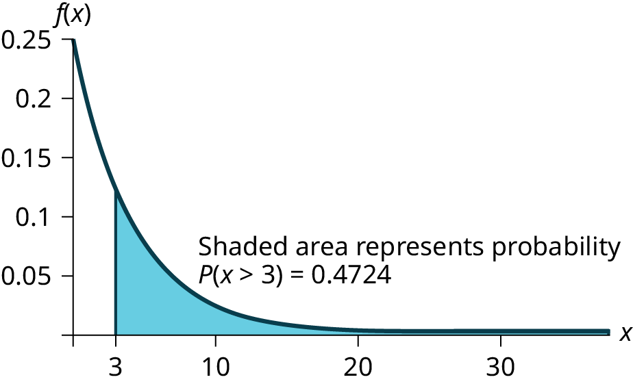
指数分布のグラフ。曲線はy軸上の点(0, 0.25)から右下がりに進み、右端でx軸に近づく。曲線の下のx = 3より右側が塗られ、P(x > 3) = 0.4724を表す。 — Figure 5.48図 5.48

Using the Calculator電卓の操作

Relationship between the Poisson and the Exponential Distributionポアソン分布と指数分布の関係

There is an interesting relationship between the exponential distribution and the Poisson distribution. Suppose that the time that elapses between two successive events follows the exponential distribution with a mean of μ units of time. Also assume that these times are independent, meaning that the time between events is not affected by the times between previous events. If these assumptions hold, then the number of events per unit time follows a Poisson distribution with mean λ = 1/μ. Recall from the chapter on Discrete Random Variables that if X has the Poisson distribution with mean λ, then

P (X = k) = \frac{λ^{k} e^{- λ}}{k!}

. Conversely, if the number of events per unit time follows a Poisson distribution, then the amount of time between events follows the exponential distribution. (k! = k*(k–1*)(k–2)*(k–3)*…3*2*1)

英語のヒント

指数分布とポアソン分布には興味深い関係がある。連続する2回の事象の間に経過する時間が、平均μ時間単位の指数分布に従うとする。また、これらの時間は独立であり、事象の発生間隔はそれ以前の発生間隔に影響されないと仮定する。これらの仮定が成り立つなら、単位時間当たりの事象の発生回数は、平均λ = 1/μのポアソン分布に従う。「離散確率変数」の章で、Xが平均λのポアソン分布に従うなら

P (X = k) = \frac{λ^{k} e^{- λ}}{k!}

となることを学んだ。逆に、単位時間当たりの発生回数がポアソン分布に従うなら、事象の発生間隔は指数分布に従う。(k! = k*(k–1*)(k–2)*(k–3)*…3*2*1)

Using the Calculator電卓の操作

Example 5.13例題 5.13

At a police station in a large city, calls come in at an average rate of four calls per minute. Assume that the time that elapses from one call to the next has the exponential distribution. Take note that we are concerned only with the rate at which calls come in, and we are ignoring the time spent on the phone. We must also assume that the times spent between calls are independent. This means that a particularly long delay between two calls does not mean that there will be a shorter waiting period for the next call. We may then deduce that the total number of calls received during a time period has the Poisson distribution.

英語のヒント

大都市のある警察署には、平均して1分に4件の電話がかかってくる。1件の電話から次の電話までの時間が指数分布に従うと仮定する。ここで考えるのは電話がかかってくる頻度だけであり、通話時間は考慮しないことに注意しよう。また、電話の間隔は独立であると仮定する必要がある。つまり、2件の電話の間隔が特に長かったからといって、次の電話までの待ち時間が短くなるわけではない。このとき、ある時間内に受ける電話の総件数はポアソン分布に従うと推論できる。

Find the average time between two successive calls.
連続する2件の電話の平均間隔を求めよ。
Find the probability that after a call is received, the next call occurs in less than ten seconds.
電話を1件受けた後、次の電話が10秒未満でかかってくる確率を求めよ。
Find the probability that exactly five calls occur within a minute.
1分間にちょうど5件の電話がかかってくる確率を求めよ。
Find the probability that less than five calls occur within a minute.
1分間にかかってくる電話が5件未満となる確率を求めよ。
Find the probability that more than 40 calls occur in an eight-minute period.
8分間に40件を超える電話がかかってくる確率を求めよ。

Solution解き方

On average there are four calls occur per minute, so 15 seconds, or $\frac{15}{60}$ = 0.25 minutes occur between successive calls on average.
平均して1分に4件かかってくるので、連続する電話の間隔は平均15秒、すなわち $\frac{15}{60}$ = 0.25分となる。
Let T = time elapsed between calls. From part a, μ = 0.25, so m = $\frac{1}{0.25}$ = 4. Thus, T ∼ Exp(4).
The cumulative distribution function is P(T < t) = 1 – e^–4t.
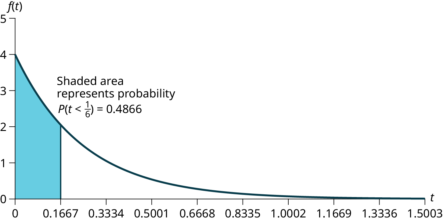
The probability that the next call occurs in less than ten seconds (ten seconds = 1/6 minute) is $P (T < \frac{1}{6}) = 1 - e^{(- 4) (\frac{1}{6})} \approx 0.4866.$
T = 電話の間に経過する時間とする。aよりμ = 0.25なので、m = $\frac{1}{0.25}$ = 4となる。したがってT ∼ Exp(4)である。累積分布関数はP(T < t) = 1 – e^–4tである。次の電話が10秒未満（10秒 = 1/6分）でかかってくる確率は $P (T < \frac{1}{6}) = 1 - e^{(- 4) (\frac{1}{6})} \approx 0.4866$ となる。

Copyright Rice University, OpenStax, Introductory Statistics 2e, CC BY 4.0. · CC BY 4.0 · Source出典

Figure 5.49図 5.49
Let X = the number of calls per minute. As previously stated, the number of calls per minute has a Poisson distribution, with a mean of four calls per minute.
Therefore, X ∼ Poisson(4), and so P(X = 5) = $\frac{4^{5} e^{- 4}}{5!}$ ≈ 0.1563. (5! = (5)(4)(3)(2)(1))
X = 1分間の電話の件数とする。先に述べたように、1分間の電話の件数は、平均4件のポアソン分布に従う。したがってX ∼ Poisson(4)であり、P(X = 5) = $\frac{4^{5} e^{- 4}}{5!}$ ≈ 0.1563となる。(5! = (5)(4)(3)(2)(1))

Using the Calculator電卓の操作

poissonpdf(4, 5) = 0.1563.
poissonpdf(4, 5) = 0.1563。
Keep in mind that X must be a whole number, so P(X < 5) = P(X ≤ 4).
To compute this, we could take P(X = 0) + P(X = 1) + P(X = 2) + P(X = 3) + P(X = 4).
Using technology, we see that P(X ≤ 4) = 0.6288.
Xは非負整数でなければならないので、P(X < 5) = P(X ≤ 4)となることに注意しよう。これはP(X = 0) + P(X = 1) + P(X = 2) + P(X = 3) + P(X = 4)によって計算できる。計算機を使うと、P(X ≤ 4) = 0.6288となる。

Using the Calculator電卓の操作

poisssoncdf(4, 4) = 0.6288
Let Y = the number of calls that occur during an eight minute period.
Since there is an average of four calls per minute, there is an average of (8)(4) = 32 calls during each eight minute period.
Hence, Y ∼ Poisson(32). Therefore, P(Y > 40) = 1 – P (Y ≤ 40) = 1 – 0.9294 = 0.0707.
Y = 8分間にかかってくる電話の件数とする。1分に平均4件なので、8分間では平均(8)(4) = 32件となる。よってY ∼ Poisson(32)である。したがって、P(Y > 40) = 1 – P(Y ≤ 40) = 1 – 0.9294 = 0.0707となる。

Using the Calculator電卓の操作

1 – poissoncdf(32, 40). = 0.0707