第26章新古典派の視点
26.1 The Building Blocks of Neoclassical Analysis26.1 新古典派の分析の基本要素
Learning Objectives学習目標
Learning Objectives学習目標
By the end of this section, you will be able to:
英語のヒント
この節を学ぶと、次のことができるようになる。
- Explain the importance of potential GDP in the long run
英語のヒント
長期における潜在GDPの重要性を説明する - Analyze the role of flexible prices
英語のヒント
柔軟な価格の役割を分析する - Interpret a neoclassical model of aggregate demand and aggregate supply
英語のヒント
総需要と総供給の新古典派モデルを読み取る - Evaluate different ways for measuring the speed of macroeconomic adjustment
英語のヒント
マクロ経済調整の速度を測るさまざまな方法を評価する
The neoclassical perspective on macroeconomics holds that, in the long run, the economy will fluctuate around its potential GDP and its natural rate of unemployment. This chapter begins with two building blocks of neoclassical economics: (1) potential GDP determines the economy's size and (2) wages and prices will adjust in a flexible manner so that the economy will adjust back to its potential GDP level of output. The key policy implication is this: The government should focus more on long-term growth and on controlling inflation than on worrying about recession or cyclical unemployment. This focus on long-run growth rather than the short-run fluctuations in the business cycle means that neoclassical economics is more useful for long-run macroeconomic analysis and Keynesian economics is more useful for analyzing the macroeconomic short run. Let's consider the two neoclassical building blocks in turn, and how we can embody them in the aggregate demand/aggregate supply model.
英語のヒント
マクロ経済の新古典派の見方では、長期には経済は潜在GDPと自然失業率の周りで変動する。本章は、新古典派経済学の二つの基本要素から始める。(1)潜在GDPが経済の規模を決める。(2)賃金と価格が柔軟に調整されるため、経済の生産は潜在GDP水準へ戻るよう調整される。重要な政策的含意は、政府は景気後退や循環的失業を心配するよりも、長期的成長とインフレ抑制に焦点を当てるべきだということだ。景気循環の短期変動より長期成長を重視するため、新古典派経済学は長期のマクロ経済分析に、ケインズ経済学は短期のマクロ経済分析に、より有用である。新古典派の二つの基本要素を順に考え、総需要・総供給モデルにどう組み込めるかを見よう。
The Importance of Potential GDP in the Long Run長期における潜在GDPの重要性
Over the long run, the level of potential GDP determines the size of real GDP. When economists refer to “potential GDP” they are referring to that level of output that an economy can achieve when all resources (land, labor, capital, and entrepreneurial ability) are fully employed. While the unemployment rate in labor markets will never be zero, full employment in the labor market refers to zero cyclical unemployment. There will still be some level of unemployment due to frictional or structural unemployment, but when the economy is operating with zero cyclical unemployment, economists say that the economy is at the natural rate of unemployment or at full employment.
英語のヒント
長期には、潜在GDPの水準が実質GDPの大きさを決める。経済学者が「潜在GDP」というとき、それはすべての資源(土地、労働、資本、企業家能力)が完全に用いられた場合に、経済が達成できる生産水準を指す。労働市場の失業率がゼロになることは決してないが、労働市場の完全雇用は循環的失業がゼロであることを指す。摩擦的・構造的失業による失業はなお残るが、経済が循環的失業ゼロで動いていれば、経済学者は自然失業率または完全雇用の状態にあるという。
Economists benchmark actual or real GDP against the potential GDP to determine how well the economy is performing. As explained in Economic Growth, we can explain GDP growth by increases in investment in physical capital and human capital per person as well as advances in technology. Physical capital per person refers to the amount and kind of machinery and equipment available to help people get work done. Compare, for example, your productivity in typing a term paper on a typewriter to working on your laptop with word processing software. Clearly, you will be able to be more productive using word processing software. The technology and level of capital of your laptop and software has increased your productivity. More broadly, the development of GPS technology and Universal Product Codes (those barcodes on every product we buy) has made it much easier for firms to track shipments, tabulate inventories, and sell and distribute products. These two technological innovations, and many others, have increased a nation's ability to produce goods and services for a given population. Likewise, increasing human capital involves increasing levels of knowledge, education, and skill sets per person through vocational or higher education. Physical and human capital improvements with technological advances will increase overall productivity and, thus, GDP.
英語のヒント
経済学者は、経済の状態を判断するため、実際のGDP、すなわち実質GDPを潜在GDPと比較する。「経済成長」で説明したように、GDP成長は、1人当たり物的資本・人的資本への投資増加と技術の進歩によって説明できる。1人当たり物的資本とは、人々の仕事を助ける機械・設備の量と種類を指す。例えば、タイプライターで学期末レポートを打つ場合と、ノートパソコンのワープロソフトで作業する場合の生産性を比べよう。明らかに、ワープロソフトを使う方が生産的になれる。ノートパソコンとソフトウェアの技術・資本水準が、生産性を高めたのである。より広く見ると、GPS技術と統一商品コード(買う製品についているバーコード)の発展によって、企業は出荷を追跡し、在庫を集計し、製品を販売・配送することがずっと容易になった。この二つの技術革新と他の多くの革新は、一定の人口で財やサービスを生産する国の能力を高めた。同様に、人的資本を増やすことは、職業教育や高等教育を通じて1人当たりの知識、教育、技能の水準を高めることである。物的資本・人的資本の改善と技術進歩は、全体の生産性を高め、GDPを増やす。
To see how these improvements have increased productivity and output at the national level, we should examine evidence from the United States. The United States experienced significant growth in the twentieth century due to phenomenal changes in infrastructure, equipment, and technological improvements in physical capital and human capital. The population more than tripled in the twentieth century, from 76 million in 1900 to over 300 million in 2016. The human capital of modern workers is far higher today because the education and skills of workers have risen dramatically. In 1900, only about one-eighth of the U.S. population had completed high school and just one person in 40 had completed a four-year college degree. By 2010, about 8.5% of Americans age 25 or older had a high school degree and about 28% had a four-year college degree as well. In 2019, 33% of Americans age 25 or older had a four-year college degree. The average amount of physical capital per worker has grown dramatically. The technology available to modern workers is extraordinarily better than a century ago: cars, airplanes, electrical machinery, smartphones, computers, chemical and biological advances, materials science, health care—the list of technological advances could run on and on. More workers, higher skill levels, larger amounts of physical capital per worker, and amazingly better technology, and potential GDP for the U.S. economy has clearly increased a great deal since 1900.
英語のヒント
これらの改善が国全体の生産性と生産をどう増やしたかを見るには、米国の証拠を調べるとよい。米国は20世紀に、インフラ、設備、物的資本と人的資本における技術の驚異的な変化によって、大きく成長した。人口は20世紀に3倍以上となり、1900年の7600万人から2016年の3億人超へ増えた。労働者の教育と技能が劇的に向上したため、現代の労働者の人的資本は今日、はるかに高い。1900年には、米国人口の約8分の1しか高校を卒業しておらず、4年制大学を卒業したのは40人に1人だけだった。2010年には、25歳以上の米国人の約8.5%が高校の卒業資格を持ち、約28%は4年制大学の学位も持っていた。2019年には、25歳以上の米国人の33%が4年制大学の学位を持っていた。労働者1人当たりの物的資本の平均量は劇的に増えた。現代の労働者が利用できる技術は、1世紀前より並外れて優れている。自動車、飛行機、電気機械、スマートフォン、コンピューター、化学・生物学の進歩、材料科学、医療など、技術進歩の例は尽きない。労働者の増加、高い技能水準、労働者1人当たり物的資本の増加、驚くほど優れた技術によって、米国経済の潜在GDPは1900年以降、明らかに大幅に増えた。
This growth has fallen below its potential GDP and, at times, has exceeded its potential. For example from 2008 to 2009, the U.S. economy tumbled into recession and remained below its potential until 2018. After the pandemic-induced recession of March and April 2020, the economy again fell below potential GDP and remains there as of early 2022. At other times, like in the late 1990s or from 2018 to 2020, the economy ran at potential GDP—or even slightly ahead. Figure 26.2 shows the actual data for the increase in real GDP since 1960. The slightly smoother line shows the potential GDP since 1960 as estimated by the nonpartisan Congressional Budget Office. Most economic recessions and upswings are times when the economy is 1–3% below or above potential GDP in a given year. Clearly, short-run fluctuations around potential GDP do exist, but over the long run, the upward trend of potential GDP determines the size of the economy.
英語のヒント
この成長は潜在GDPを下回ることも、時には潜在水準を超えることもあった。例えば2008~2009年、米国経済は景気後退に落ち込み、2018年まで潜在水準を下回り続けた。2020年3月・4月のパンデミックによる景気後退の後、経済は再び潜在GDPを下回り、2022年初めにもそこにとどまっている。1990年代後半や2018~2020年のように、潜在GDP、さらにはそれをわずかに上回る水準で動いた時期もある。図26.2は1960年以降の実質GDPの増加の実際のデータを示す。やや滑らかな線は、超党派の議会予算局が推定した1960年以降の潜在GDPである。大半の景気後退や上昇局面は、その年の経済が潜在GDPを1~3%下回るか上回る時期である。明らかに潜在GDPの周りに短期変動は存在するが、長期には潜在GDPの上昇傾向が経済の大きさを決める。
Potential and Actual GDP (in 2012 Dollars), 1958–2020潜在GDPと実際のGDP(2012年ドル)、1958~2020年
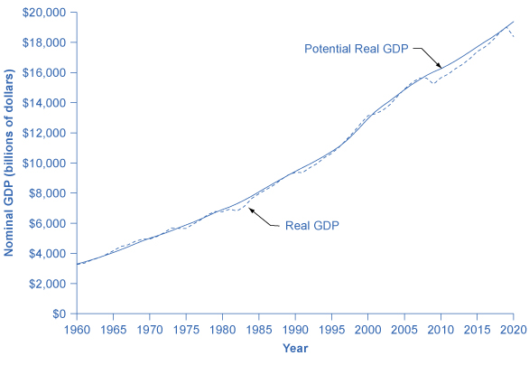
Figure 26.2図 26.2
Actual GDP falls below potential GDP during and after recessions, like the recessions of 1980 and 1981–82, 1990–91, 2001, and 2008–2009 and continues below potential GDP until 2019, when it goes slightly above potential. In other cases, actual GDP can be above potential GDP for a time, as in the late 1990s.
英語のヒント
実際のGDPは、1980年と1981~1982年、1990~1991年、2001年、2008~2009年のような景気後退の間とその後に潜在GDPを下回り、2019年にわずかに上回るまで潜在GDP未満にとどまる。他の場合には、1990年代後半のように、一時的に実際のGDPが潜在GDPを上回ることもある。
In the aggregate demand/aggregate supply model, we show potential GDP as a vertical line. Neoclassical economists who focus on potential GDP as the primary determinant of real GDP argue that the long-run aggregate supply curve is located at potential GDP—that is, we draw the long-run aggregate supply curve as a vertical line at the level of potential GDP, as Figure 26.3 shows. A vertical LRAS curve means that the level of aggregate supply (or potential GDP) will determine the economy's real GDP, regardless of the level of aggregate demand. Over time, increases in the quantity and quality of physical capital, increases in human capital, and technological advancements shift potential GDP and the vertical LRAS curve gradually to the right. Economists often describe this gradual increase in an economy's potential GDP as a nation's long-term economic growth.
英語のヒント
総需要・総供給モデルでは、潜在GDPを垂直線で示す。実質GDPの主要な決定要因として潜在GDPに注目する新古典派の経済学者は、長期総供給曲線が潜在GDPに位置すると論じる。つまり図26.3のように、潜在GDP水準の垂直線として長期総供給曲線を描く。垂直なLRAS曲線は、総需要の水準にかかわらず、総供給(または潜在GDP)の水準が経済の実質GDPを決めることを意味する。時間とともに、物的資本の量と質の向上、人的資本の増加、技術進歩によって、潜在GDPと垂直なLRAS曲線は徐々に右へシフトする。経済学者は、経済の潜在GDPのこの緩やかな増加を、国の長期的経済成長と呼ぶことが多い。
A Vertical AS Curve垂直なAS曲線
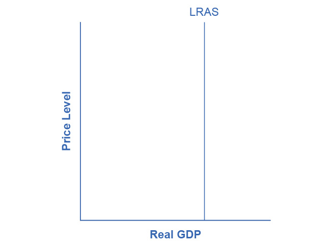


Figure 26.3図 26.3
In the neoclassical model, we draw the aggregate supply curve as a vertical line at the level of potential GDP. If AS is vertical, then it determines the level of real output, no matter where we draw the aggregate demand curve. Over time, the LRAS curve shifts to the right as productivity increases and potential GDP expands.
英語のヒント
新古典派モデルでは、潜在GDP水準の垂直線として総供給曲線を描く。ASが垂直なら、総需要曲線をどこに描いても、ASが実質生産水準を決める。生産性が高まり潜在GDPが拡大するにつれ、LRAS曲線は時間とともに右へシフトする。