第4章微分の応用

The Second Derivative Test第2次導関数による極値の判定

The first derivative test provides an analytical tool for finding local extrema, but the second derivative can also be used to locate extreme values. Using the second derivative can sometimes be a simpler method than using the first derivative.

第1次導関数による判定は、計算で極値を求める方法であるが、第2次導関数でも極値を調べられる。場合によっては、第2次導関数を使うほうが簡単になる。

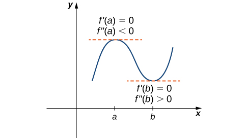
We know that if a continuous function has local extrema, it must occur at a critical point. However, a function need not have local extrema at a critical point. Here we examine how the second derivative test can be used to determine whether a function has a local extremum at a critical point. Let

f

be a twice-differentiable function such that

f^{'} (a) = 0

and

f^{″}

is continuous over an open interval

I

containing

a .

Suppose

f^{″} (a) < 0 .

Since

f^{″}

is continuous over

I,

f^{″} (x) < 0

for all

x \in I

(Figure 4.38). Then, by Corollary

3,

f^{'}

is a decreasing function over

I .

Since

f^{'} (a) = 0,

we conclude that for all

x \in I, f^{'} (x) > 0

x < a

and

f^{'} (x) < 0

x > a .

Therefore, by the first derivative test,

f

has a local maximum at

x = a .

On the other hand, suppose there exists a point

b

such that

f^{'} (b) = 0

but

f^{″} (b) > 0 .

Since

f^{″}

is continuous over an open interval

I

containing

b,

then

f^{″} (x) > 0

for all

x \in I

(Figure 4.38). Then, by Corollary

3, f^{'}

is an increasing function over

I .

Since

f^{'} (b) = 0,

we conclude that for all

x \in I,

f^{'} (x) < 0

x < b

and

f^{'} (x) > 0

x > b .

Therefore, by the first derivative test,

f

has a local minimum at

x = b .

連続関数が極値をとるなら、その位置は臨界点である。しかし、臨界点で必ず極値をとるとは限らない。ここでは、第2次導関数を使って判定する方法を考える。

f

を2回微分可能な関数とし、

f^{'} (a) = 0

とする。また、

f^{″}

は

a

を含む開区間

I

で連続であるとする。

f^{″} (a) < 0

なら、

f^{″}

の連続性により、

I

を必要に応じて十分小さく取り直すことで、すべての

x \in I

について

f^{″} (x) < 0

とできる（図4.38）。系

3

から、

f^{'}

は

I

上で減少する。

f^{'} (a) = 0

なので、

x < a

の側では

f' (x) > 0

であり、

x > a

の側では

f^{'} (x) < 0

である。よって、第1次導関数による判定から、

f

は

x = a

で極大値をとる。一方、

f^{'} (b) = 0

かつ

f^{″} (b) > 0

となる点

b

があるとしよう。

f^{″}

が

b

を含む開区間

I

で連続なら、区間を十分小さく取ることで、すべての

x \in I

で

f^{″} (x) > 0

となる（図4.38）。すると、系

3

より、f′は

I

上で増加する。

f^{'} (b) = 0

なので、

x \in I

について、

x < b

なら

f^{'} (x) < 0

、

x > b

なら

f^{'} (x) > 0

である。第1次導関数による判定から、

f

は

x = b

で極小値をとる。

関数f(x)はx=aまで増加し、その後x=bまで減少してから再び増加する。極大点(a,f(a))でf′(a)=0、f″(a)<0。極小点(b,f(b))でf′(b)=0、f″(b)>0。 — Figure 4.38図 4.38
Consider a twice-differentiable function $f$ such that $f^{″}$ is continuous. Since $f' (a) = 0$ and $f^{″} (a) < 0,$ there is an interval $I$ containing $a$ such that for all $x$ in $I,$ $f$ is increasing if $x < a$ and $f$ is decreasing if $x > a .$ As a result, $f$ has a local maximum at $x = a .$ Since $f' (b) = 0$ and $f^{″} (b) > 0,$ there is an interval $I$ containing $b$ such that for all $x$ in $I,$ $f$ is decreasing if $x < b$ and $f$ is increasing if $x > b .$ As a result, $f$ has a local minimum at $x = b .$
$f$ を2回微分可能な関数とし、 $f^{″}$ が連続であるとする。 $f' (a) = 0$ かつ $f^{″} (a) < 0$ なら、 $a$ を含む区間 $I$ が存在し、 $I$ 内の $x$ について、 $x < a$ なら $f$ は増加し、 $x > a$ なら $f$ は減少する。よって、 $f$ は $x = a$ で極大値をとる。 $f' (b) = 0$ かつ $f^{″} (b) > 0$ なら、 $b$ を含む区間 $I$ が存在し、 $I$ 内の $x$ について、 $x < b$ なら $f$ は減少し、 $x > b$ なら $f$ は増加する。よって、 $f$ は $x = b$ で極小値をとる。

Note that for case iii. when

f^{″} (c) = 0,

then

f

may have a local maximum, local minimum, or neither at

c .

For example, the functions

f (x) = x^{3},

f (x) = x^{4},

and

f (x) = − x^{4}

all have critical points at

x = 0 .

In each case, the second derivative is zero at

x = 0 .

However, the function

f (x) = x^{4}

has a local minimum at

x = 0

whereas the function

f (x) = − x^{4}

has a local maximum at

x = 0

and the function

f (x) = x^{3}

does not have a local extremum at

x = 0 .

英語のヒント

(iii)の

f^{″} (c) = 0

の場合、

f

は

c

で極大値をとることも、極小値をとることも、どちらもとらないこともある。例えば

f (x) = x^{3}

、

f (x) = x^{4}

、

f (x) = − x^{4}

は、どれも

x = 0

に臨界点をもち、

x = 0

で第2次導関数が0になる。それでも、

f (x) = x^{4}

は

x = 0

で極小値をとり、

f (x) = − x^{4}

は

x = 0

で極大値をとる。一方、

f (x) = x^{3}

は

x = 0

で極値をとらない。

Let’s now look at how to use the second derivative test to determine whether

f

has a local maximum or local minimum at a critical point

c

where

f^{'} (c) = 0 .

f^{'} (c) = 0

となる臨界点

c

で、

f

が極大値・極小値をとるかどうかを、第2次導関数で判定する例を見よう。

Example 4.20例題 4.20

Using the Second Derivative Test第2次導関数による判定を使う

Use the second derivative to find the location of all local extrema for

f (x) = x^{5} - 5 x^{3} .

第2次導関数を用いて、

f (x) = x^{5} - 5 x^{3}

が極値をとる位置をすべて求めよ。

Solution解き方

To apply the second derivative test, we first need to find critical points

c

where

f^{'} (c) = 0 .

The derivative is

f^{'} (x) = 5 x^{4} - 15 x^{2} .

Therefore,

f^{'} (x) = 5 x^{4} - 15 x^{2} = 5 x^{2} (x^{2} - 3) = 0

when

x = 0, ± \sqrt{3} .

第2次導関数による判定を使うには、まず

f^{'} (c) = 0

を満たす臨界点

c

を求める。導関数は

f^{'} (x) = 5 x^{4} - 15 x^{2}

である。したがって、

x = 0, ± \sqrt{3}

のとき

f^{'} (x) = 5 x^{4} - 15 x^{2} = 5 x^{2} (x^{2} - 3) = 0

となる。

To determine whether

f

has local extrema at any of these points, we need to evaluate the sign of

f^{″}

at these points. The second derivative is

これらの点で

f

が極値をとるかを判定するため、それぞれの点で

f^{″}

の符号を調べる。第2次導関数は、

f^{″} (x) = 20 x^{3} - 30 x = 10 x (2 x^{2} - 3) .

f^{″} (x) = 20 x^{3} - 30 x = 10 x (2 x^{2} - 3)

In the following table, we evaluate the second derivative at each of the critical points and use the second derivative test to determine whether

f

has a local maximum or local minimum at any of these points.

次の表では、各臨界点で第2次導関数の値を求め、第2次導関数による判定から、

f

が極大値・極小値をとるかを調べる。

$x$	$f^{″} (x)$	Conclusion 結論
$− \sqrt{3}$	$−30 \sqrt{3}$	Local maximum 極大
$0$	$0$	Second derivative test is inconclusive 第2次導関数による判定では結論が出ない
$\sqrt{3}$	$30 \sqrt{3}$	Local minimum 極小

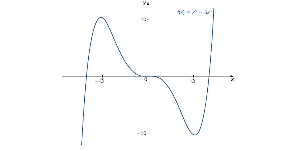
By the second derivative test, we conclude that

f

has a local maximum at

x = − \sqrt{3}

and

f

has a local minimum at

x = \sqrt{3} .

The second derivative test is inconclusive at

x = 0 .

To determine whether

f

has local extrema at

x = 0,

we apply the first derivative test. To evaluate the sign of

f^{'} (x) = 5 x^{2} (x^{2} - 3)

for

x \in (− \sqrt{3}, 0)

and

x \in (0, \sqrt{3}),

let

x = −1

and

x = 1

be the two test points. Since

f^{'} (−1) < 0

and

f^{'} (1) < 0,

we conclude that

f

is decreasing on both intervals and, therefore,

f

does not have local extrema at

x = 0

as shown in the following graph.

第2次導関数による判定から、

f

は

x = − \sqrt{3}

で極大値をとり、

f

は

x = \sqrt{3}

で極小値をとる。一方、

x = 0

では、この方法だけで結論を出せない。

f

が

x = 0

で極値をとるかを調べるため、第1次導関数による判定を使う。

x \in (− \sqrt{3}, 0)

と

x \in (0, \sqrt{3})

で

f^{'} (x) = 5 x^{2} (x^{2} - 3)

の符号を調べるため、試験点として

x = −1

と

x = 1

を選ぶ。

f^{'} (−1) < 0

かつ

f^{'} (1) < 0

なので、

f

は両区間で減少する。したがって、

f

は

x = 0

で極値をとらない。次のグラフもこの結果を示している。

f(x)=x⁵−5x³のグラフ。x=−√3で極大値6√3（約10.39）をとるまで増加し、その後減少する。原点は接線が水平な変曲点で、そのまま減少が続く。x=√3で極小値−6√3（約−10.39）をとり、その後増加する。 — Figure 4.39図 4.39
The function $f$ has a local maximum at $x = − \sqrt{3}$ and a local minimum at $x = \sqrt{3}$
関数 $f$ は $x = − \sqrt{3}$ で極大値、 $x = \sqrt{3}$ で極小値をとる。

We have now developed the tools we need to determine where a function is increasing and decreasing, as well as acquired an understanding of the basic shape of the graph. In the next section we discuss what happens to a function as

x \to ± \infty .

At that point, we have enough tools to provide accurate graphs of a large variety of functions.

英語のヒント

関数がどこで増加・減少するかを判定する方法と、グラフの基本的な形の調べ方が揃った。次の節では、

x \to ± \infty

のときの関数の振る舞いを学ぶ。そこまで進めば、さまざまな関数のグラフを正確に描くための道具が揃う。