第4章微分の応用

Determining End Behavior for Transcendental Functions超越関数の無限遠での振る舞い

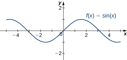
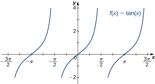
The six basic trigonometric functions are periodic and do not approach a finite limit as

x \to ± \infty .

For example,

sin x

oscillates between

1 and −1

(Figure 4.58). The tangent function

x

has an infinite number of vertical asymptotes as

x \to ± \infty;

therefore, it does not approach a finite limit nor does it approach

± \infty

x \to ± \infty

as shown in Figure 4.59.

基本的な六つの三角関数は周期関数であり、

x \to ± \infty

のとき有限の極限値へ近づかない。例えば、

sin x

は

1 と −1

の間を振動する（図4.58）。正接関数tan

x

には、

x \to ± \infty

に向かう途中に垂直漸近線が無数にある。したがって、

x \to ± \infty

のとき有限の極限値へ近づくことも、

± \infty

へ発散することもない（図4.59）。

f(x)=sin xのグラフ。−1と1の間を周期的に振動し続ける。 — Figure 4.58図 4.58
The function $f (x) = sin x$ oscillates between $1 and −1$ as $x \to ± \infty$
関数 $f (x) = sin x$ は、 $x \to ± \infty$ のときも $1 と −1$ の間を振動し続ける。

f(x)=tan xのグラフ。各枝は垂直漸近線の間で負の無限大から正の無限大へ増加する。この形が繰り返される。 — Figure 4.59図 4.59
The function $f (x) = tan x$ does not approach a limit and does not approach $± \infty$ as $x \to ± \infty$
関数 $f (x) = tan x$ は、 $x \to ± \infty$ のとき有限の極限値へ近づかず、 $± \infty$ へ発散することもない。

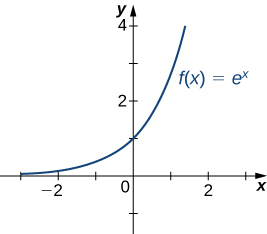
Recall that for any base

b > 0, b \neq 1,

the function

y = b^{x}

is an exponential function with domain

(− \infty, \infty)

and range

(0, \infty) .

b > 1, y = b^{x}

is increasing over

(− \infty, \infty) .

0 < b < 1,

y = b^{x}

is decreasing over

(− \infty, \infty) .

For the natural exponential function

f (x) = e^{x},

e \approx 2.718 > 1 .

Therefore,

f (x) = e^{x}

is increasing on

(− \infty, \infty)

and the range is

(0, \infty) .

The exponential function

f (x) = e^{x}

approaches

\infty

x \to \infty

and approaches

0

x \to − \infty

as shown in Table 4.5 and Figure 4.60.

底が

b > 0, b \neq 1

を満たすとき、

y = b^{x}

は定義域が

(− \infty, \infty)

、値域が

(0, \infty)

の指数関数である。

b > 1

y = b^{x}

は

(− \infty, \infty)

で増加する。

0 < b < 1

なら、

y = b^{x}

は

(− \infty, \infty)

で減少する。自然指数関数

f (x) = e^{x}

では、

e \approx 2.718 > 1

である。したがって、

f (x) = e^{x}

は

(− \infty, \infty)

で増加し、値域は

(0, \infty)

となる。指数関数

f (x) = e^{x}

は、

x \to \infty

のとき

\infty

へ発散し、

x \to − \infty

のとき

0

へ近づく。表4.5と図4.60を参照。

End behavior of the natural exponential function自然指数関数の無限遠での振る舞い

Table 4.5表 4.5
$x$	$−5$	$−2$	$0$	$2$	$5$
$e^{x}$	$0.00674$	$0.135$	$1$	$7.389$	$148.413$

f(x)=eˣのグラフ。常に正で、(0,1)を通って増加する。左の遠方では0へ近づき、右の遠方では正の無限大へ発散する。 — Figure 4.60図 4.60
The exponential function approaches zero as $x \to − \infty$ and approaches $\infty$ as $x \to \infty .$
指数関数は、 $x \to − \infty$ のとき0へ近づき、 $x \to \infty$ のとき $\infty$ へ発散する。

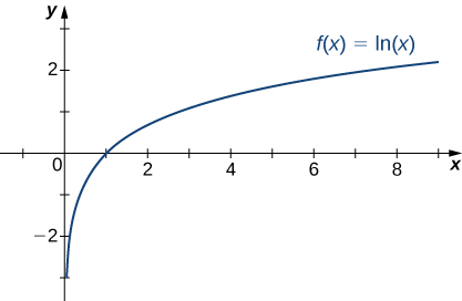
Recall that the natural logarithm function

f (x) = ln (x)

is the inverse of the natural exponential function

y = e^{x} .

Therefore, the domain of

f (x) = ln (x)

(0, \infty)

and the range is

(− \infty, \infty) .

The graph of

f (x) = ln (x)

is the reflection of the graph of

y = e^{x}

about the line

y = x .

Therefore,

ln (x) \to − \infty

x \to 0^{+}

and

ln (x) \to \infty

x \to \infty

as shown in Figure 4.61 and Table 4.6.

自然対数関数

f (x) = ln (x)

は、自然指数関数

y = e^{x}

の逆関数である。そのため、

f (x) = ln (x)

の定義域は

(0, \infty)

、値域は

(− \infty, \infty)

となる。

f (x) = ln (x)

のグラフは、

y = e^{x}

のグラフを直線

y = x

に関して対称移動したものである。したがって、

x \to 0^{+}

のとき

ln (x) \to − \infty

となり、

x \to \infty

のとき

ln (x) \to \infty

となる。図4.61と表4.6を参照。

End behavior of the natural logarithm function自然対数関数の端での振る舞い

Table 4.6表 4.6
$x$	$0.01$	$0.1$	$1$	$10$	$100$
$ln (x)$	$−4.605$	$−2.303$	$0$	$2.303$	$4.605$

f(x)=ln xのグラフ。定義域はx>0。(1,0)を通って増加し、x→0⁺では負の無限大、x→∞では正の無限大へ向かう。 — Figure 4.61図 4.61
The natural logarithm function approaches $\infty$ as $x \to \infty .$
自然対数関数は、 $x \to \infty$ のとき $\infty$ へ発散する。

Example 4.27例題 4.27

Determining End Behavior for a Transcendental Function超越関数の無限遠での振る舞いを調べる

Find the limits as

x \to \infty

and

x \to − \infty

for

f (x) = \frac{(2 + 3 e^{x})}{(7 - 5 e^{x})}

and describe the end behavior of

f .

f (x) = \frac{(2 + 3 e^{x})}{(7 - 5 e^{x})}

について、

x \to \infty

と

x \to − \infty

のときの極限を求め、

f

の無限遠での振る舞いを説明せよ。

Solution解き方

To find the limit as

x \to \infty,

divide the numerator and denominator by

e^{x} :

x \to \infty

のときの極限を求めるため、分子と分母を

e^{x} :

で割る。

\begin{matrix} lim_{x \to \infty} f (x) & = lim_{x \to \infty} \frac{2 + 3 e^{x}}{7 - 5 e^{x}} \\ = lim_{x \to \infty} \frac{(2 / e^{x}) + 3}{(7 / e^{x}) - 5} . \end{matrix}

As shown in Figure 4.60,

e^{x} \to \infty

x \to \infty .

Therefore,

図4.60のとおり、

x \to \infty

のとき

e^{x} \to \infty

となる。したがって、

lim_{x \to \infty} \frac{2}{e^{x}} = 0 = lim_{x \to \infty} \frac{7}{e^{x}} .

lim_{x \to \infty} \frac{2}{e^{x}} = 0 = lim_{x \to \infty} \frac{7}{e^{x}}

We conclude that

lim_{x \to \infty} f (x) = - \frac{3}{5},

and the graph of

f

approaches the horizontal asymptote

y = - \frac{3}{5}

x \to \infty .

To find the limit as

x \to − \infty,

use the fact that

e^{x} \to 0

x \to − \infty

to conclude that

lim_{x \to - \infty} f (x) = \frac{2}{7},

and therefore the graph of approaches the horizontal asymptote

y = \frac{2}{7}

x \to − \infty .

よって、

lim_{x \to \infty} f (x) = - \frac{3}{5}

であり、

x \to \infty

のとき

f

のグラフは水平漸近線

y = - \frac{3}{5}

へ近づく。

x \to − \infty

のときの極限は、

x \to − \infty

なら

e^{x} \to 0

となることを使って求めると、

lim_{x \to - \infty} f (x) = \frac{2}{7}

である。したがって、

x \to − \infty

のとき、このグラフは水平漸近線

y = \frac{2}{7}

へ近づく。

Guidelines for Drawing the Graph of a Function関数のグラフを描くための指針

We now have enough analytical tools to draw graphs of a wide variety of algebraic and transcendental functions. Before showing how to graph specific functions, let’s look at a general strategy to use when graphing any function.

英語のヒント

これまでに、さまざまな代数関数や超越関数のグラフを描くための道具が揃った。個々の関数を描く前に、一般的に使える手順を整理しよう。

Drawing the Graph of a Function関数のグラフを描く

Given a function

f,

use the following steps to sketch a graph of

f :

関数

f

が与えられたら、次の手順で

f :

のグラフの概形を描く。

Determine the domain of the function.
関数の定義域を求める。
Locate the $x$ - and $y$ -intercepts.
$x$ 切片と $y$ 切片を求める。
Evaluate $lim_{x \to \infty} f (x)$ and $lim_{x \to − \infty} f (x)$ to determine the end behavior. If either of these limits is a finite number $L,$ then $y = L$ is a horizontal asymptote. If either of these limits is $\infty$ or $− \infty,$ determine whether $f$ has an oblique asymptote. If $f$ is a rational function such that $f (x) = \frac{p (x)}{q (x)},$ where the degree of the numerator is greater than the degree of the denominator, then $f$ can be written as
$lim_{x \to \infty} f (x)$ と $lim_{x \to − \infty} f (x)$ を求め、無限遠での振る舞いを調べる。どちらかの極限が有限の数 $L$ なら、 $y = L$ は水平漸近線である。どちらかの極限が $\infty$ または $− \infty$ なら、 $f$ に斜漸近線があるか調べる。 $f$ が有理関数 $f (x) = \frac{p (x)}{q (x)}$ で、分子の次数が分母の次数より大きい場合、 $f$ は次のように書ける。

$f (x) = \frac{p (x)}{q (x)} = g (x) + \frac{r (x)}{q (x)},$
$f (x) = \frac{p (x)}{q (x)} = g (x) + \frac{r (x)}{q (x)}$

where the degree of $r (x)$ is less than the degree of $q (x) .$ The values of $f (x)$ approach the values of $g (x)$ as $x \to ± \infty .$ If $g (x)$ is a linear function, it is known as an oblique asymptote.
ここで、 $r (x)$ の次数は $q (x)$ の次数より小さい。 $x \to ± \infty$ のとき、 $f (x)$ と $g (x)$ の値の差は0へ近づく。 $g (x)$ が1次関数なら、そのグラフは斜漸近線である。
Determine whether $f$ has any vertical asymptotes.
$f$ に垂直漸近線があるか調べる。
Calculate $f^{'} .$ Find all critical points and determine the intervals where $f$ is increasing and where $f$ is decreasing. Determine whether $f$ has any local extrema.
$f^{'}$ を計算する。すべての臨界点を求め、 $f$ が増加する区間と $f$ が減少する区間を調べる。 $f$ が極大値・極小値をもつか判定する。
Calculate $f^{″} .$ Determine the intervals where $f$ is concave up and where $f$ is concave down. Use this information to determine whether $f$ has any inflection points. The second derivative can also be used as an alternate means to determine or verify that $f$ has a local extremum at a critical point.
$f^{″}$ を計算する。 $f$ が下に凸となる区間と、 $f$ が上に凸となる区間を調べ、それを使って $f$ に変曲点があるか判定する。第2次導関数は、臨界点で $f$ が極値をもつかを判定したり、既に求めた極値を確認したりする別の方法としても使える。

Now let’s use this strategy to graph several different functions. We start by graphing a polynomial function.

この手順で、いくつかの関数のグラフを描こう。まず、多項式関数から始める。

Example 4.28例題 4.28

Sketching a Graph of a Polynomial多項式関数のグラフの概形を描く

Sketch a graph of

f (x) = {(x - 1)}^{2} (x + 2) .

f (x) = {(x - 1)}^{2} (x + 2)

のグラフの概形を描け。

Solution解き方

Step 1. Since

f

is a polynomial, the domain is the set of all real numbers.

手順1．

f

は多項式なので、定義域は実数全体である。

Step 2. When

x = 0, f (x) = 2 .

Therefore, the

y

-intercept is

(0, 2) .

To find the

x

-intercepts, we need to solve the equation

{(x - 1)}^{2} (x + 2) = 0,

gives us the

x

-intercepts

(1, 0)

and

(−2, 0)

手順2．

x = 0

f (x) = 2

なので、

y

切片は

(0, 2)

である。

x

切片を求めるには、方程式

{(x - 1)}^{2} (x + 2) = 0

を解く。その結果、

x

切片は

(1, 0)

と

(−2, 0)

である。

Step 3. We need to evaluate the end behavior of

f .

x \to \infty,

{(x - 1)}^{2} \to \infty

and

(x + 2) \to \infty .

Therefore,

lim_{x \to \infty} f (x) = \infty .

x \to − \infty,

{(x - 1)}^{2} \to \infty

and

(x + 2) \to − \infty .

Therefore,

lim_{x \to − \infty} f (x) = − \infty .

To get even more information about the end behavior of

f,

we can multiply the factors of

f .

When doing so, we see that

手順3．

f

の無限遠での振る舞いを調べる。

x \to \infty

のとき、

{(x - 1)}^{2} \to \infty

かつ

(x + 2) \to \infty

なので、

lim_{x \to \infty} f (x) = \infty

となる。

x \to − \infty

のとき、

{(x - 1)}^{2} \to \infty

かつ

(x + 2) \to − \infty

なので、

lim_{x \to − \infty} f (x) = − \infty

となる。

f

の無限遠での振る舞いをさらに詳しく調べるため、

f

の因子を掛けて展開すると、

f (x) = {(x - 1)}^{2} (x + 2) = x^{3} - 3 x + 2 .

f (x) = {(x - 1)}^{2} (x + 2) = x^{3} - 3 x + 2

Since the leading term of

f

x^{3},

we conclude that

f

behaves like

y = x^{3}

x \to ± \infty .

f

の最高次の項は

x^{3}

なので、

x \to ± \infty

のとき

f

は

y = x^{3}

と同じ向きに発散し、主要な増大率も等しい。

Step 4. Since

f

is a polynomial function, it does not have any vertical asymptotes.

手順4．

f

は多項式関数なので、垂直漸近線をもたない。

Step 5. The first derivative of

f

手順5．

f

の第1次導関数は、

f^{'} (x) = 3 x^{2} - 3 .

f^{'} (x) = 3 x^{2} - 3

Therefore,

f

has two critical points:

x = 1, −1 .

Divide the interval

(− \infty, \infty)

into the three smaller intervals:

(− \infty, −1),

(−1, 1),

and

(1, \infty) .

Then, choose test points

x = −2,

x = 0,

and

x = 2

from these intervals and evaluate the sign of

f^{'} (x)

at each of these test points, as shown in the following table.

したがって、

f

には

x = 1, −1

という二つの臨界点がある。区間

(− \infty, \infty)

を、

(− \infty, −1)

、

(−1, 1)

、

(1, \infty)

の三つに分ける。各区間から調べる点として

x = −2

、

x = 0

、

x = 2

を選び、それぞれで

f^{'} (x)

の符号を調べる。結果を次の表に示す。

Interval 区間	Test Point 調べる点	Sign of Derivative $f' (x) = 3 x^{2} - 3 = 3 (x - 1) (x + 1)$ 導関数 $f' (x) = 3 x^{2} - 3 = 3 (x - 1) (x + 1)$ の符号	Conclusion 結論
$(− \infty, −1)$	$x = −2$	$(+) (−) (−) = +$	$f$ is increasing. $f$ は増加している。
$(−1, 1)$	$x = 0$	$(+) (−) (+) = −$	$f$ is decreasing. $f$ は減少している。
$(1, \infty)$	$x = 2$	$(+) (+) (+) = +$	$f$ is increasing. $f$ は増加している。

From the table, we see that

f

has a local maximum at

x = −1

and a local minimum at

x = 1 .

Evaluating

f (x)

at those two points, we find that the local maximum value is

f (−1) = 4

and the local minimum value is

f (1) = 0 .

表から、

f

は

x = −1

で極大値、

x = 1

で極小値をとる。この2点で

f (x)

を計算すると、極大値は

f (−1) = 4

、極小値は

f (1) = 0

である。

Step 6. The second derivative of

f

手順6．

f

の第2次導関数は、

f^{″} (x) = 6 x .

f^{″} (x) = 6 x

The second derivative is zero at

x = 0 .

Therefore, to determine the concavity of

f,

divide the interval

(− \infty, \infty)

into the smaller intervals

(− \infty, 0)

and

(0, \infty),

and choose test points

x = −1

and

x = 1

to determine the concavity of

f

on each of these smaller intervals as shown in the following table.

第2次導関数は

x = 0

で0になる。そこで

f

の凹凸を調べるため、区間

(− \infty, \infty)

を

(− \infty, 0)

と

(0, \infty)

に分ける。各区間から

x = −1

と

x = 1

を選び、そこでの符号から各区間における

f

の凹凸を判定する。結果を次の表に示す。

Interval 区間	Test Point 調べる点	Sign of $f^{″} (x) = 6 x$ $f^{″} (x) = 6 x$ の符号	Conclusion 結論
$(− \infty, 0)$	$x = −1$	$-$	$f$ is concave down. $f$ は上に凸である。
$(0, \infty)$	$x = 1$	$+$	$f$ is concave up. $f$ は下に凸である。

We note that the information in the preceding table confirms the fact, found in step

5,

that

f

has a local maximum at

x = −1

and a local minimum at

x = 1 .

In addition, the information found in step

5

—namely,

f

has a local maximum at

x = −1

and a local minimum at

x = 1,

and

f^{'} (x) = 0

at those points—combined with the fact that

f^{″}

changes sign only at

x = 0

confirms the results found in step

6

on the concavity of

f .

直前の表は、手順

5

で求めた「

f

が

x = −1

で極大値、

x = 1

で極小値をとる」という結果も裏付ける。これらの点では第2次導関数がそれぞれ負・正だからである。逆に、手順

5

で得た「

f

は

x = −1

で極大、

x = 1

で極小となり、両点で

f^{'} (x) = 0

である」という結果と、この例では第2次導関数が両点で0でなく、

f^{″}

の符号が変わるのは

x = 0

だけであることを合わせても、手順

6

の

f

の凹凸を確認できる。

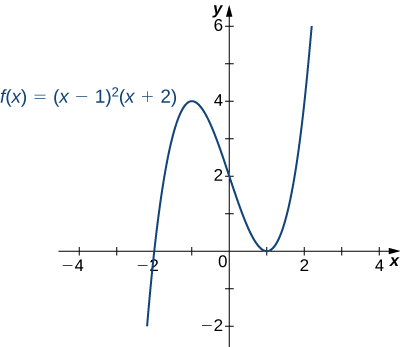
Combining this information, we arrive at the graph of

f (x) = {(x - 1)}^{2} (x + 2)

shown in the following graph.

以上をまとめると、

f (x) = {(x - 1)}^{2} (x + 2)

のグラフは次のようになる。

f(x)=(x−1)²(x+2)のグラフ。x=−2でx軸を横切り、x=1でx軸に接する。極大点は(−1,4)、極小点は(1,0)である。

OpenStax, Rice University; Calculus Volume 1. · CC BY-NC-SA 4.0

Example 4.29例題 4.29

Sketching a Rational Function有理関数のグラフの概形を描く

Sketch the graph of

f (x) = \frac{x^{2}}{(1 - x^{2})} .

f (x) = \frac{x^{2}}{(1 - x^{2})} .

のグラフの概形を描け。

Solution解き方

Step 1. The function

f

is defined as long as the denominator is not zero. Therefore, the domain is the set of all real numbers

x

except

x = ± 1 .

手順1．

f

は分母が0でない限り定義される。したがって、定義域は

x = ± 1

を除くすべての実数

x

である。

Step 2. Find the intercepts. If

x = 0,

then

f (x) = 0,

0

is an intercept. If

y = 0,

then

\frac{x^{2}}{(1 - x^{2})} = 0,

which implies

x = 0 .

Therefore,

(0, 0)

is the only intercept.

手順2．切片を求める。

x = 0

なら

f (x) = 0

なので、y切片は

0

である。

y = 0

なら

\frac{x^{2}}{(1 - x^{2})} = 0

であり、ここから

x = 0

となる。したがって、座標軸との交点は

(0, 0)

だけである。

Step 3. Evaluate the limits at infinity. Since

f

is a rational function, divide the numerator and denominator by the highest power in the denominator:

x^{2} .

We obtain

手順3．無限遠での極限を求める。

f

は有理関数なので、分子と分母を、分母の最高の累乗

x^{2}

で割る。すると、

lim_{x \to ± \infty} \frac{x^{2}}{1 - x^{2}} = lim_{x \to ± \infty} \frac{1}{\frac{1}{x^{2}} - 1} = −1 .

lim_{x \to ± \infty} \frac{x^{2}}{1 - x^{2}} = lim_{x \to ± \infty} \frac{1}{\frac{1}{x^{2}} - 1} = −1

Therefore,

f

has a horizontal asymptote of

y = −1

x \to \infty

and

x \to − \infty .

したがって、

f

は、

x \to \infty

と

x \to − \infty

の両方で、水平漸近線

y = −1

をもつ。

Step 4. To determine whether

f

has any vertical asymptotes, first check to see whether the denominator has any zeroes. We find the denominator is zero when

x = ± 1 .

To determine whether the lines

x = 1

x = −1

are vertical asymptotes of

f,

evaluate

lim_{x \to 1} f (x)

and

lim_{x \to − 1} f (x) .

By looking at each one-sided limit as

x \to 1,

we see that

手順4．

f

に垂直漸近線があるか調べるため、まず分母が0になる点を探す。その点は

x = ± 1

である。直線

x = 1

と

x = −1

が

f

の垂直漸近線かどうかを判定するため、

lim_{x \to 1} f (x)

と

lim_{x \to − 1} f (x)

を調べる。

x \to 1

の左右からの極限を見ると、

lim_{x \to 1^{+}} \frac{x^{2}}{1 - x^{2}} = − \infty and lim_{x \to 1^{-}} \frac{x^{2}}{1 - x^{2}} = \infty .

lim_{x \to 1^{+}} \frac{x^{2}}{1 - x^{2}} = − \infty および lim_{x \to 1^{-}} \frac{x^{2}}{1 - x^{2}} = \infty

In addition, by looking at each one-sided limit as

x \to − 1,

we find that

さらに、

x \to − 1

の左右からの極限を見ると、

lim_{x \to − 1^{+}} \frac{x^{2}}{1 - x^{2}} = \infty and lim_{x \to − 1^{-}} \frac{x^{2}}{1 - x^{2}} = − \infty .

lim_{x \to − 1^{+}} \frac{x^{2}}{1 - x^{2}} = \infty および lim_{x \to − 1^{-}} \frac{x^{2}}{1 - x^{2}} = − \infty

Step 5. Calculate the first derivative:

手順5．第1次導関数を計算する。

f^{'} (x) = \frac{(1 - x^{2}) (2 x) - x^{2} (−2 x)}{{(1 - x^{2})}^{2}} = \frac{2 x}{{(1 - x^{2})}^{2}} .

f^{'} (x) = \frac{(1 - x^{2}) (2 x) - x^{2} (−2 x)}{{(1 - x^{2})}^{2}} = \frac{2 x}{{(1 - x^{2})}^{2}}

Critical points occur at points

x

where

f^{'} (x) = 0

f^{'} (x)

is undefined. We see that

f^{'} (x) = 0

when

x = 0 .

The derivative

f^{'}

is not undefined at any point in the domain of

f .

However,

x = ± 1

are not in the domain of

f .

Therefore, to determine where

f

is increasing and where

f

is decreasing, divide the interval

(− \infty, \infty)

into four smaller intervals:

(− \infty, −1),

(−1, 0),

(0, 1),

and

(1, \infty),

and choose a test point in each interval to determine the sign of

f^{'} (x)

in each of these intervals. The values

x = −2,

x = - \frac{1}{2},

x = \frac{1}{2},

and

x = 2

are good choices for test points as shown in the following table.

臨界点は、定義域内で

f^{'} (x) = 0

となるか、

f^{'} (x)

が定義されない点

x

である。ここでは、

x = 0

のとき

f^{'} (x) = 0

となる。

f

の定義域内には

f^{'}

が定義されない点はない。

x = ± 1

は

f

の定義域に含まれない。それも考慮して、

f

が増加する区間と

f

が減少する区間を調べるため、

(− \infty, \infty)

を

(− \infty, −1)

、

(−1, 0)

、

(0, 1)

、

(1, \infty)

に分ける。各区間で一点ずつ選び、

f^{'} (x)

の符号を調べる。例えば

x = −2

、

x = - \frac{1}{2}

、

x = \frac{1}{2}

、

x = 2

を選ぶと、次の表が得られる。

Interval 区間	Test Point 調べる点	Sign of $f^{'} (x) = \frac{2 x}{{(1 - x^{2})}^{2}}$ $f^{'} (x) = \frac{2 x}{{(1 - x^{2})}^{2}}$ の符号	Conclusion 結論
$(− \infty, −1)$	$x = −2$	$− / + = −$	$f$ is decreasing. $f$ は減少している。
$(−1, 0)$	$x = −1 / 2$	$− / + = −$	$f$ is decreasing. $f$ は減少している。
$(0, 1)$	$x = 1 / 2$	$+ / + = +$	$f$ is increasing. $f$ は増加している。
$(1, \infty)$	$x = 2$	$+ / + = +$	$f$ is increasing. $f$ は増加している。

From this analysis, we conclude that

f

has a local minimum at

x = 0

but no local maximum.

以上より、

f

は

x = 0

で極小値をとるが、極大値はもたない。

Step 6. Calculate the second derivative:

手順6．第2次導関数を計算する。

\begin{matrix} f^{″} (x) & = \frac{{(1 - x^{2})}^{2} (2) - 2 x (2 (1 - x^{2}) (−2 x))}{{(1 - x^{2})}^{4}} \\ = \frac{(1 - x^{2}) [2 (1 - x^{2}) + 8 x^{2}]}{{(1 - x^{2})}^{4}} \\ = \frac{2 (1 - x^{2}) + 8 x^{2}}{{(1 - x^{2})}^{3}} \\ = \frac{6 x^{2} + 2}{{(1 - x^{2})}^{3}} . \end{matrix}

To determine the intervals where

f

is concave up and where

f

is concave down, we first need to find all points

x

where

f^{″} (x) = 0

f^{″} (x)

is undefined. Since the numerator

6 x^{2} + 2 \neq 0

for any

x,

f^{″} (x)

is never zero. Furthermore,

f^{″}

is not undefined for any

x

in the domain of

f .

However, as discussed earlier,

x = ± 1

are not in the domain of

f .

Therefore, to determine the concavity of

f,

we divide the interval

(− \infty, \infty)

into the three smaller intervals

(− \infty, −1),

(−1, 1),

and

(1, \infty),

and choose a test point in each of these intervals to evaluate the sign of

f^{″} (x) .

in each of these intervals. The values

x = −2,

x = 0,

and

x = 2

are possible test points as shown in the following table.

f

が下に凸となる区間と

f

が上に凸となる区間を調べるため、まず

f^{″} (x) = 0

となるか

f^{″} (x)

が定義されない点

x

を探す。どの

x

についても分子は

6 x^{2} + 2 \neq 0

なので、

f^{″} (x)

は0にならない。また、

f

の定義域内のどの

x

でも、

f^{″}

は定義される。既に述べたように、

x = ± 1

は

f

の定義域に含まれない。

f

の凹凸を調べるため、

(− \infty, \infty)

を

(− \infty, −1)

、

(−1, 1)

、

(1, \infty)

に分け、各区間で一点ずつ選んで

f^{″} (x)

の符号を調べる。例えば

x = −2

、

x = 0

、

x = 2

を選ぶと、次の表が得られる。

Interval 区間	Test Point 調べる点	Sign of $f^{″} (x) = \frac{6 x^{2} + 2}{{(1 - x^{2})}^{3}}$ $f^{″} (x) = \frac{6 x^{2} + 2}{{(1 - x^{2})}^{3}}$ の符号	Conclusion 結論
$(− \infty, −1)$	$x = −2$	$+ / - = −$	$f$ is concave down. $f$ は上に凸である。
$(−1, −1)$	$x = 0$	$+ / + = +$	$f$ is concave up. $f$ は下に凸である。
$(1, \infty)$	$x = 2$	$+ / - = −$	$f$ is concave down. $f$ は上に凸である。

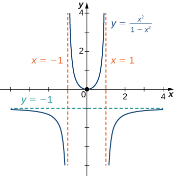
Combining all this information, we arrive at the graph of

f

shown below. Note that, although

f

changes concavity at

x = −1

and

x = 1,

there are no inflection points at either of these places because

f

is not continuous at

x = −1

x = 1 .

以上をまとめると、

f

のグラフは次のようになる。

f

は

x = −1

と

x = 1

を境に凹凸が変わるが、どちらにも変曲点はない。

f

は

x = −1

でも

x = 1

でも連続ではなく、そもそもそこで定義されないからである。

f(x)=x²/(1−x²)のグラフ。漸近線はy=−1、x=−1、x=1。区間(−1,1)では下に凸で、原点が極小点。左右の外側では上に凸である。

OpenStax, Rice University; Calculus Volume 1. · CC BY-NC-SA 4.0

Example 4.30例題 4.30

Sketching a Rational Function with an Oblique Asymptote斜漸近線をもつ有理関数のグラフ

Sketch the graph of

f (x) = \frac{x^{2}}{(x - 1)}

f (x) = \frac{x^{2}}{(x - 1)}

のグラフの概形を描け。

Solution解き方

Step 1. The domain of

f

is the set of all real numbers

x

except

x = 1 .

手順1．

f

の定義域は、

x = 1

を除くすべての実数

x

である。

Step 2. Find the intercepts. We can see that when

x = 0,

f (x) = 0,

(0, 0)

is the only intercept.

手順2．切片を求める。

x = 0

のとき

f (x) = 0

であり、分子が0になるのもこのときだけなので、座標軸との交点は

(0, 0)

だけである。

Step 3. Evaluate the limits at infinity. Since the degree of the numerator is one more than the degree of the denominator,

f

must have an oblique asymptote. To find the oblique asymptote, use long division of polynomials to write

手順3．無限遠での極限を求める。分子の次数が分母の次数より1大きいので、

f

は斜漸近線をもつ。多項式の割り算を使って、

f (x) = \frac{x^{2}}{x - 1} = x + 1 + \frac{1}{x - 1} .

f (x) = \frac{x^{2}}{x - 1} = x + 1 + \frac{1}{x - 1}

Since

1 / (x - 1) \to 0

x \to ± \infty,

f (x)

approaches the line

y = x + 1

x \to ± \infty .

The line

y = x + 1

is an oblique asymptote for

f .

x \to ± \infty

のとき

1 / (x - 1) \to 0

なので、

x \to ± \infty

のとき

f (x)

は直線

y = x + 1

へ近づく。直線

y = x + 1

が

f

の斜漸近線である。

Step 4. To check for vertical asymptotes, look at where the denominator is zero. Here the denominator is zero at

x = 1 .

Looking at both one-sided limits as

x \to 1,

we find

手順4．垂直漸近線を調べるため、分母が0になる点を探す。ここでは

x = 1

である。

x \to 1

の左右からの極限を調べると、

lim_{x \to 1^{+}} \frac{x^{2}}{x - 1} = \infty and lim_{x \to 1^{-}} \frac{x^{2}}{x - 1} = − \infty .

lim_{x \to 1^{+}} \frac{x^{2}}{x - 1} = \infty および lim_{x \to 1^{-}} \frac{x^{2}}{x - 1} = − \infty

Therefore,

x = 1

is a vertical asymptote, and we have determined the behavior of

f

x

approaches

1

from the right and the left.

したがって、

x = 1

は垂直漸近線である。これで、

x

が

1

へ右から、また左から近づくときの

f

の振る舞いも分かった。

Step 5. Calculate the first derivative:

手順5．第1次導関数を計算する。

f^{'} (x) = \frac{(x - 1) (2 x) - x^{2} (1)}{{(x - 1)}^{2}} = \frac{x^{2} - 2 x}{{(x - 1)}^{2}} .

f^{'} (x) = \frac{(x - 1) (2 x) - x^{2} (1)}{{(x - 1)}^{2}} = \frac{x^{2} - 2 x}{{(x - 1)}^{2}}

We have

f^{'} (x) = 0

when

x^{2} - 2 x = x (x - 2) = 0 .

Therefore,

x = 0

and

x = 2

are critical points. Since

f

is undefined at

x = 1,

we need to divide the interval

(− \infty, \infty)

into the smaller intervals

(− \infty, 0),

(0, 1),

(1, 2),

and

(2, \infty),

and choose a test point from each interval to evaluate the sign of

f^{'} (x)

in each of these smaller intervals. For example, let

x = −1,

x = \frac{1}{2},

x = \frac{3}{2},

and

x = 3

be the test points as shown in the following table.

x^{2} - 2 x = x (x - 2) = 0

のとき

f^{'} (x) = 0

となるので、

x = 0

と

x = 2

が臨界点である。

f

は

x = 1

で定義されないことも考慮する。

(− \infty, \infty)

を

(− \infty, 0)

、

(0, 1)

、

(1, 2)

、

(2, \infty)

に分け、各区間から一点ずつ選んで

f^{'} (x)

の符号を調べる。例えば

x = −1

、

x = \frac{1}{2}

、

x = \frac{3}{2}

、

x = 3

を選ぶと、次の表が得られる。

Interval 区間	Test Point 調べる点	Sign of $f' (x) = \frac{x^{2} - 2 x}{{(x - 1)}^{2}} = \frac{x (x - 2)}{{(x - 1)}^{2}}$ $f' (x) = \frac{x^{2} - 2 x}{{(x - 1)}^{2}} = \frac{x (x - 2)}{{(x - 1)}^{2}}$ の符号	Conclusion 結論
$(− \infty, 0)$	$x = −1$	$(−) (−) / + = +$	$f$ is increasing. $f$ は増加している。
$(0, 1)$	$x = 1 / 2$	$(+) (−) / + = −$	$f$ is decreasing. $f$ は減少している。
$(1, 2)$	$x = 3 / 2$	$(+) (−) / + = −$	$f$ is decreasing. $f$ は減少している。
$(2, \infty)$	$x = 3$	$(+) (+) / + = +$	$f$ is increasing. $f$ は増加している。

From this table, we see that

f

has a local maximum at

x = 0

and a local minimum at

x = 2 .

The value of

f

at the local maximum is

f (0) = 0

and the value of

f

at the local minimum is

f (2) = 4 .

Therefore,

(0, 0)

and

(2, 4)

are important points on the graph.

この表から、

f

は

x = 0

で極大値、

x = 2

で極小値をとる。

f

の極大値は

f (0) = 0

、

f

の極小値は

f (2) = 4

である。したがって、

(0, 0)

と

(2, 4)

はグラフを描くうえで重要な点となる。

Step 6. Calculate the second derivative:

手順6．第2次導関数を計算する。

\begin{matrix} f^{″} (x) & = \frac{{(x - 1)}^{2} (2 x - 2) - (x^{2} - 2 x) (2 (x - 1))}{{(x - 1)}^{4}} \\ = \frac{(x - 1) [(x - 1) (2 x - 2) - 2 (x^{2} - 2 x)]}{{(x - 1)}^{4}} \\ = \frac{(x - 1) (2 x - 2) - 2 (x^{2} - 2 x)}{{(x - 1)}^{3}} \\ = \frac{2 x^{2} - 4 x + 2 - (2 x^{2} - 4 x)}{{(x - 1)}^{3}} \\ = \frac{2}{{(x - 1)}^{3}} . \end{matrix}

We see that

f^{″} (x)

is never zero or undefined for

x

in the domain of

f .

Since

f

is undefined at

x = 1,

to check concavity we just divide the interval

(− \infty, \infty)

into the two smaller intervals

(− \infty, 1)

and

(1, \infty),

and choose a test point from each interval to evaluate the sign of

f^{″} (x)

in each of these intervals. The values

x = 0

and

x = 2

are possible test points as shown in the following table.

f

の定義域内の

x

について、

f^{″} (x)

は0にも未定義にもならない。

f

は

x = 1

で定義されないので、凹凸を調べるには、

(− \infty, \infty)

を

(− \infty, 1)

と

(1, \infty)

に分ければよい。各区間から一点ずつ選び、

f^{″} (x)

の符号を調べる。例えば

x = 0

と

x = 2

を選ぶと、次の表が得られる。

Interval 区間	Test Point 調べる点	Sign of $f^{″} (x) = \frac{2}{{(x - 1)}^{3}}$ $f^{″} (x) = \frac{2}{{(x - 1)}^{3}}$ の符号	Conclusion 結論
$(− \infty, 1)$	$x = 0$	$+ / - = −$	$f$ is concave down. $f$ は上に凸である。
$(1, \infty)$	$x = 2$	$+ / + = +$	$f$ is concave up. $f$ は下に凸である。

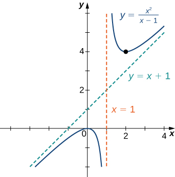
From the information gathered, we arrive at the following graph for

f .

以上の情報から、

f

のグラフは次のようになる。

f(x)=x²/(x−1)のグラフ。斜漸近線はy=x+1、垂直漸近線はx=1。極大点は(0,0)、極小点は(2,4)である。

OpenStax, Rice University; Calculus Volume 1. · CC BY-NC-SA 4.0

Example 4.31例題 4.31

Sketching the Graph of a Function with a Cusp尖点をもつ関数のグラフ

Sketch a graph of

f (x) = {(x - 1)}^{2 / 3} .

f (x) = {(x - 1)}^{2 / 3}

のグラフの概形を描け。

Solution解き方

Step 1. Since the cube-root function is defined for all real numbers

x

and

{(x - 1)}^{2 / 3} = {(\sqrt[3]{x - 1})}^{2},

the domain of

f

is all real numbers.

手順1．立方根はすべての実数

x

について定義され、

{(x - 1)}^{2 / 3} = {(\sqrt[3]{x - 1})}^{2}

である。したがって、

f

の定義域は実数全体である。

Step 2: To find the

y

-intercept, evaluate

f (0) .

Since

f (0) = 1,

the

y

-intercept is

(0, 1) .

To find the

x

-intercept, solve

{(x - 1)}^{2 / 3} = 0 .

The solution of this equation is

x = 1,

so the

x

-intercept is

(1, 0) .

手順2．

y

切片を求めるため、

f (0)

を計算する。

f (0) = 1

なので、

y

切片は

(0, 1)

である。

x

切片を求めるには、

{(x - 1)}^{2 / 3} = 0

を解く。解は

x = 1

なので、

x

切片は

(1, 0)

である。

Step 3: Since

lim_{x \to ± \infty} {(x - 1)}^{2 / 3} = \infty,

the function continues to grow without bound as

x \to \infty

and

x \to − \infty .

手順3．

lim_{x \to ± \infty} {(x - 1)}^{2 / 3} = \infty

なので、

x \to \infty

のときも

x \to − \infty

のときも、関数の値は限りなく大きくなる。

Step 4: The function has no vertical asymptotes.

手順4．この関数には垂直漸近線がない。

Step 5: To determine where

f

is increasing or decreasing, calculate

f^{'} .

We find

手順5．

f

の増減を調べるため、

f^{'}

を計算する。すると、

f^{'} (x) = \frac{2}{3} {(x - 1)}^{−1 / 3} = \frac{2}{3 {(x - 1)}^{1 / 3}} .

f^{'} (x) = \frac{2}{3} {(x - 1)}^{−1 / 3} = \frac{2}{3 {(x - 1)}^{1 / 3}}

This function is not zero anywhere, but it is undefined when

x = 1 .

Therefore, the only critical point is

x = 1 .

Divide the interval

(− \infty, \infty)

into the smaller intervals

(− \infty, 1)

and

(1, \infty),

and choose test points in each of these intervals to determine the sign of

f^{'} (x)

in each of these smaller intervals. Let

x = 0

and

x = 2

be the test points as shown in the following table.

この導関数はどこでも0にならないが、

x = 1

で定義されない。したがって、唯一の臨界点は

x = 1

である。

(− \infty, \infty)

を

(− \infty, 1)

と

(1, \infty)

に分け、各区間で一点ずつ選んで

f^{'} (x)

の符号を調べる。

x = 0

と

x = 2

を選ぶと、次の表が得られる。

Interval 区間	Test Point 調べる点	Sign of $f^{'} (x) = \frac{2}{3 {(x - 1)}^{1 / 3}}$ $f^{'} (x) = \frac{2}{3 {(x - 1)}^{1 / 3}}$ の符号	Conclusion 結論
$(− \infty, 1)$	$x = 0$	$+ / - = −$	$f$ is decreasing. $f$ は減少している。
$(1, \infty)$	$x = 2$	$+ / + = +$	$f$ is increasing. $f$ は増加している。

We conclude that

f

has a local minimum at

x = 1 .

Evaluating

f

x = 1,

we find that the value of

f

at the local minimum is zero. Note that

f^{'} (1)

is undefined, so to determine the behavior of the function at this critical point, we need to examine

lim_{x \to 1} f^{'} (x) .

Looking at the one-sided limits, we have

以上より、

f

は

x = 1

で極小値をとる。

x = 1

における

f

を計算すると、

f

の極小値は0である。

f^{'} (1)

は定義されないので、この臨界点でのグラフの形を詳しく知るには、

lim_{x \to 1} f^{'} (x)

を調べる必要がある。左右からの極限は、

lim_{x \to 1^{+}} \frac{2}{3 {(x - 1)}^{1 / 3}} = \infty and lim_{x \to 1^{-}} \frac{2}{3 {(x - 1)}^{1 / 3}} = − \infty .

lim_{x \to 1^{+}} \frac{2}{3 {(x - 1)}^{1 / 3}} = \infty および lim_{x \to 1^{-}} \frac{2}{3 {(x - 1)}^{1 / 3}} = − \infty

Therefore,

f

has a cusp at

x = 1 .

したがって、

f

は

x = 1

に尖点をもつ。

Step 6: To determine concavity, we calculate the second derivative of

f :

手順6．凹凸を調べるため、

f :

の第2次導関数を計算する。

f^{″} (x) = - \frac{2}{9} {(x - 1)}^{−4 / 3} = \frac{−2}{9 {(x - 1)}^{4 / 3}} .

f^{″} (x) = - \frac{2}{9} {(x - 1)}^{−4 / 3} = \frac{−2}{9 {(x - 1)}^{4 / 3}}

We find that

f^{″} (x)

is defined for all

x,

but is undefined when

x = 1 .

Therefore, divide the interval

(− \infty, \infty)

into the smaller intervals

(− \infty, 1)

and

(1, \infty),

and choose test points to evaluate the sign of

f^{″} (x)

in each of these intervals. As we did earlier, let

x = 0

and

x = 2

be test points as shown in the following table.

f^{″} (x)

は

x = 1

では定義されず、それ以外のすべての

x

で定義される。そこで、

(− \infty, \infty)

を

(− \infty, 1)

と

(1, \infty)

に分け、各区間で

f^{″} (x)

の符号を調べる。先ほどと同じく、調べる点を

x = 0

と

x = 2

に選ぶと、次の表が得られる。

Interval 区間	Test Point 調べる点	Sign of $f^{″} (x) = \frac{−2}{9 {(x - 1)}^{4 / 3}}$ $f^{″} (x) = \frac{−2}{9 {(x - 1)}^{4 / 3}}$ の符号	Conclusion 結論
$(− \infty, 1)$	$x = 0$	$− / + = −$	$f$ is concave down. $f$ は上に凸である。
$(1, \infty)$	$x = 2$	$− / + = −$	$f$ is concave down. $f$ は上に凸である。

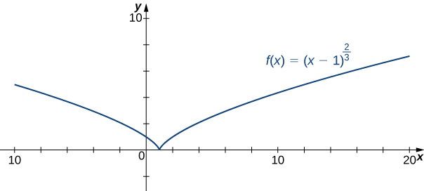
From this table, we conclude that

f

is concave down everywhere. Combining all of this information, we arrive at the following graph for

f .

表から、

f

は尖点の左側・右側の各区間で上に凸である。以上をまとめると、

f

のグラフは次のようになる。

f(x)=(x−1)^(2/3)のグラフ。(1,0)に尖点があり、そこから左右へ上方に広がる。尖点の両側ではそれぞれ上に凸である。

OpenStax, Rice University; Calculus Volume 1. · CC BY-NC-SA 4.0

Checkpoint 4.30確認問題 4.30

Consider the function

f (x) = 5 - x^{2 / 3} .

Determine the point on the graph where a cusp is located. Determine the end behavior of

f .

関数

f (x) = 5 - x^{2 / 3}

を考える。グラフ上の尖点の座標と、

f

の無限遠での振る舞いを求めよ。

Solution解き方

The function

f

has a cusp at

(0, 5)

lim_{x \to 0^{-}} f^{'} (x) = \infty,

lim_{x \to 0^{+}} f^{'} (x) = − \infty .

For end behavior,

lim_{x \to ± \infty} f (x) = − \infty .

関数

f

は

(0, 5)

に尖点をもつ。

lim_{x \to 0^{-}} f^{'} (x) = \infty

であり、

lim_{x \to 0^{+}} f^{'} (x) = − \infty

である。無限遠での振る舞いは、

lim_{x \to ± \infty} f (x) = − \infty

である。