第4章微分の応用

4.6 Limits at Infinity and Asymptotes4.6　無限遠での極限と漸近線

Learning Objectives学習目標

Calculate the limit of a function as $x$ increases or decreases without bound.
$x$ が正または負の方向へ限りなく進むときの関数の極限を計算する。
Recognize a horizontal asymptote on the graph of a function.
関数のグラフの水平漸近線を見つける。
Estimate the end behavior of a function as $x$ increases or decreases without bound.
$x$ が正または負の方向へ限りなく進むときの関数の振る舞いを推定する。
Recognize an oblique asymptote on the graph of a function.
関数のグラフの斜漸近線を見つける。
Analyze a function and its derivatives to draw its graph.
関数とその導関数を調べ、グラフを描く。

We have shown how to use the first and second derivatives of a function to describe the shape of a graph. To graph a function

f

defined on an unbounded domain, we also need to know the behavior of

f

x \to ± \infty .

In this section, we define limits at infinity and show how these limits affect the graph of a function. At the end of this section, we outline a strategy for graphing an arbitrary function

f .

英語のヒント

第1次・第2次導関数を使ってグラフの形を調べる方法を学んだ。有界でない定義域をもつ関数

f

のグラフを描くには、

x \to ± \infty

のときの

f

の振る舞いも知る必要がある。この節では無限遠での極限を定義し、それがグラフの形とどう関わるかを調べる。最後に、任意の関数

f

のグラフを描く手順をまとめる。

Limits at Infinity無限遠での極限

We begin by examining what it means for a function to have a finite limit at infinity. Then we study the idea of a function with an infinite limit at infinity. Back in Introduction to Functions and Graphs, we looked at vertical asymptotes; in this section we deal with horizontal and oblique asymptotes.

英語のヒント

まず、無限遠で関数が有限の極限をもつとはどういうことかを考える。その後、無限遠で関数の値が無限大へ発散する場合を学ぶ。「関数とグラフへの導入」では垂直漸近線を扱った。この節では、水平漸近線と斜めの漸近線を扱う。

Limits at Infinity and Horizontal Asymptotes無限遠での極限と水平漸近線

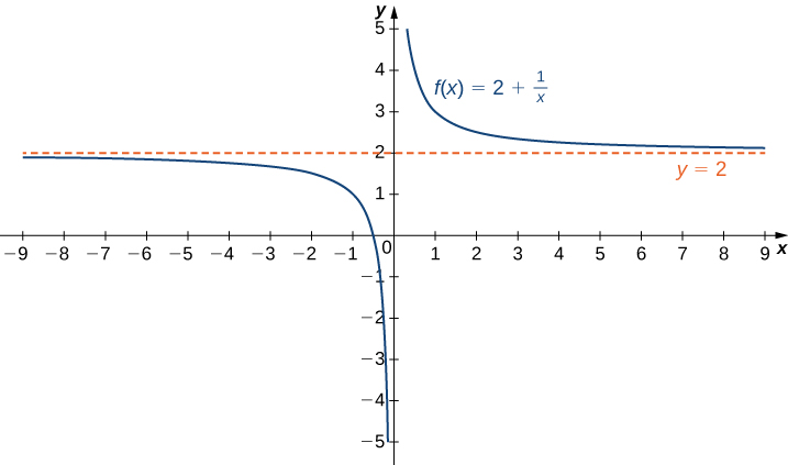
Recall that

lim_{x \to a} f (x) = L

means

f (x)

becomes arbitrarily close to

L

as long as

x

is sufficiently close to

a .

We can extend this idea to limits at infinity. For example, consider the function

f (x) = 2 + \frac{1}{x} .

As can be seen graphically in Figure 4.40 and numerically in Table 4.2, as the values of

x

get larger, the values of

f (x)

approach

2 .

We say the limit as

x

approaches

\infty

f (x)

2

and write

lim_{x \to \infty} f (x) = 2 .

Similarly, for

x < 0,

as the values

| x |

get larger, the values of

f (x)

approaches

2 .

We say the limit as

x

approaches

− \infty

f (x)

2

and write

lim_{x \to - \infty} f (x) = 2 .

英語のヒント

lim_{x \to a} f (x) = L

とは、

x

を

a

へ十分近づければ、

f (x)

を

L

へ望むだけ近づけられる、という意味だった。この考え方を、無限遠での極限へ広げられる。例えば

f (x) = 2 + \frac{1}{x}

を考えよう。図4.40と表4.2から、

x

が大きくなるにつれて

f (x)

は

2 .

へ近づくと分かる。これを、

x

が

\infty

に近づくときの

f (x)

の極限は

2

であるといい、

lim_{x \to \infty} f (x) = 2

と書く。同様に、

x < 0

のもとで

| x |

を大きくすると、

f (x)

は

2 .

へ近づく。これを、

x

が

− \infty

に近づくときの

f (x)

の極限は

2

であるといい、

lim_{x \to - \infty} f (x) = 2

と書く。

f(x)=2+1/xのグラフ。x<0の枝は、左の遠方ではy=2の下側に近く、xを0に近づけると負の無限大へ下がる。x>0の枝は、0の右側では正の無限大から下がり、右の遠方ではy=2の上側へ近づく。水平漸近線y=2が描かれている。 — Figure 4.40図 4.40
The function approaches the asymptote $y = 2$ as $x$ approaches $± \infty .$
$x$ が $± \infty$ へ近づくと、関数のグラフは漸近線 $y = 2$ へ近づく。

Values of a function $f$ as $x \to ± \infty$ $x \to ± \infty$ のときの関数 $f$ の値

Table 4.2表 4.2
$x$	$10$	$100$	$1,000$	$10,000$
$2 + \frac{1}{x}$	$2.1$	$2.01$	$2.001$	$2.0001$
$x$	$−10$	$−100$	$−1000$	$−10,000$
$2 + \frac{1}{x}$	$1.9$	$1.99$	$1.999$	$1.9999$

More generally, for any function

f,

we say the limit as

x \to \infty

f (x)

L

f (x)

becomes arbitrarily close to

L

as long as

x

is sufficiently large. In that case, we write

lim_{x \to \infty} f (x) = L .

Similarly, we say the limit as

x \to − \infty

f (x)

L

f (x)

becomes arbitrarily close to

L

as long as

x < 0

and

| x |

is sufficiently large. In that case, we write

lim_{x \to − \infty} f (x) = L .

We now look at the definition of a function having a limit at infinity.

一般に、関数

f

について、

x

を十分大きくすれば

f (x)

を

L

へ望むだけ近づけられるとする。このとき、

x \to \infty

における

f (x)

の極限は

L

であるといい、

lim_{x \to \infty} f (x) = L

と書く。同様に、

x < 0

で

| x |

を十分大きくすれば、

f (x)

を

L

へ望むだけ近づけられるとする。このとき、

x \to − \infty

における

f (x)

の極限は

L

であるといい、

lim_{x \to − \infty} f (x) = L

と書く。無限遠で極限をもつことを、次のように定義しよう。

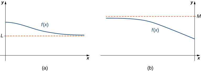
If the values

f (x)

are getting arbitrarily close to some finite value

L

x \to \infty

x \to − \infty,

the graph of

f

approaches the line

y = L .

In that case, the line

y = L

is a horizontal asymptote of

f

(Figure 4.41). For example, for the function

f (x) = \frac{1}{x},

since

lim_{x \to \infty} f (x) = 0,

the line

y = 0

is a horizontal asymptote of

f (x) = \frac{1}{x} .

x \to \infty

または

x \to − \infty

のときに、

f (x)

がある有限の値

L

へ望むだけ近づくなら、

f

のグラフは直線

y = L

へ近づく。この直線

y = L

を、

f

の水平漸近線という（図4.41）。例えば、関数

f (x) = \frac{1}{x}

では

lim_{x \to \infty} f (x) = 0

なので、直線

y = 0

は

f (x) = \frac{1}{x}

の水平漸近線である。

二つの水平漸近線の例。(a) 右の遠方でf(x)が上側から高さLの水平な破線へ近づく。(b) 左の遠方でf(x)が下側から高さMの水平な破線へ近づく。 — Figure 4.41図 4.41
(a) As $x \to \infty,$ the values of $f$ are getting arbitrarily close to $L .$ The line $y = L$ is a horizontal asymptote of $f .$ (b) As $x \to − \infty,$ the values of $f$ are getting arbitrarily close to $M .$ The line $y = M$ is a horizontal asymptote of $f .$
(a) $x \to \infty$ のとき、 $f$ の値は $L$ へ望むだけ近づく。直線 $y = L$ は $f$ の水平漸近線である。(b) $x \to − \infty$ のとき、 $f$ の値は $M$ へ望むだけ近づく。直線 $y = M$ は $f$ の水平漸近線である。

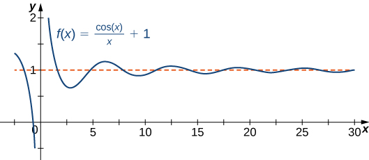
A function cannot cross a vertical asymptote because the graph must approach infinity (or

− \infty)

from at least one direction as

x

approaches the vertical asymptote. However, a function may cross a horizontal asymptote. In fact, a function may cross a horizontal asymptote an unlimited number of times. For example, the function

f (x) = \frac{(cos x)}{x} + 1

shown in Figure 4.42 intersects the horizontal asymptote

y = 1

an infinite number of times as it oscillates around the asymptote with ever-decreasing amplitude.

英語のヒント

x

が垂直漸近線へ近づくとき、少なくとも一方の側では、関数値が正の無限大または

- \infty

へ発散する。そのため、有限の高さを保った連続な曲線として垂直漸近線を横切ることはできない。一方、グラフが水平漸近線と交わることはある。無限回交わることさえある。例えば、図4.42の関数

f (x) = \frac{(cos x)}{x} + 1

は、振幅を次第に小さくしながら

y = 1

の周りで振動し、この水平漸近線と無限回交わる。

f(x)=(cos x)/x+1の正のx側のグラフ。0の右側では非常に大きく、そこから減少する。その後はy=1の周りを、振幅を小さくしながら振動する。 — Figure 4.42図 4.42
The graph of $f (x) = (cos x) / x + 1$ crosses its horizontal asymptote $y = 1$ an infinite number of times.
$f (x) = (cos x) / x + 1$ のグラフは、水平漸近線 $y = 1$ と無限回交わる。

The algebraic limit laws and squeeze theorem we introduced in Introduction to Limits also apply to limits at infinity. We illustrate how to use these laws to compute several limits at infinity.

「極限への導入」で学んだ極限の演算法則とはさみうちの定理は、無限遠での極限にも適用できる。これらを使って、いくつかの極限を計算しよう。

Example 4.21例題 4.21

Computing Limits at Infinity無限遠での極限を計算する

For each of the following functions

f,

evaluate

lim_{x \to \infty} f (x)

and

lim_{x \to − \infty} f (x) .

Determine the horizontal asymptote(s) for

f .

次の各関数

f

について、

lim_{x \to \infty} f (x)

と

lim_{x \to − \infty} f (x)

を求めよ。また、

f

の水平漸近線を求めよ。

$f (x) = 5 - \frac{2}{x^{2}}$
$f (x) = 5 - \frac{2}{x^{2}}$
$f (x) = \frac{sin x}{x}$
$f (x) = \frac{sin x}{x}$
$f (x) = {tan}^{−1} (x)$
$f (x) = {tan}^{−1} (x)$

Solution解き方

Using the algebraic limit laws, we have $lim_{x \to \infty} (5 - \frac{2}{x^{2}}) = lim_{x \to \infty} 5 - 2 (lim_{x \to \infty} \frac{1}{x}) . (lim_{x \to \infty} \frac{1}{x}) = 5 - 2 \cdot 0 = 5 .$
Similarly, $lim_{x \to - \infty} f (x) = 5 .$ Therefore, $f (x) = 5 - \frac{2}{x^{2}}$ has a horizontal asymptote of $y = 5$ and $f$ approaches this horizontal asymptote as $x \to ± \infty$ as shown in the following graph.
極限の演算法則を使うと、 $lim_{x \to \infty} (5 - \frac{2}{x^{2}}) = lim_{x \to \infty} 5 - 2 (lim_{x \to \infty} \frac{1}{x}) . (lim_{x \to \infty} \frac{1}{x}) = 5 - 2 \cdot 0 = 5$ となる。同様に、 $lim_{x \to - \infty} f (x) = 5$ である。したがって、 $f (x) = 5 - \frac{2}{x^{2}}$ の水平漸近線は $y = 5$ であり、 $f$ は $x \to ± \infty$ のとき、この水平漸近線へ近づく。次のグラフを参照。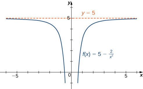

OpenStax, Rice University; Calculus Volume 1. · CC BY-NC-SA 4.0

Figure 4.43図 4.43
This function approaches a horizontal asymptote as $x \to ± \infty .$
この関数は、 $x \to ± \infty$ のときに水平漸近線へ近づく。
Since $−1 \leq sin x \leq 1$ for all $x,$ we have
すべての $x$ で $−1 \leq sin x \leq 1$ なので、

$\frac{−1}{x} \leq \frac{sin x}{x} \leq \frac{1}{x}$

for all $x \neq 0 .$ Also, since
これはすべての $x \neq 0$ について成り立つ。また、

$lim_{x \to \infty} \frac{−1}{x} = 0 = lim_{x \to \infty} \frac{1}{x},$
$lim_{x \to \infty} \frac{−1}{x} = 0 = lim_{x \to \infty} \frac{1}{x}$

we can apply the squeeze theorem to conclude that
したがって、はさみうちの定理を適用すると、

$lim_{x \to \infty} \frac{sin x}{x} = 0 .$
$lim_{x \to \infty} \frac{sin x}{x} = 0$

Similarly,
同様に、

$lim_{x \to − \infty} \frac{sin x}{x} = 0 .$
$lim_{x \to − \infty} \frac{sin x}{x} = 0$

Thus, $f (x) = \frac{sin x}{x}$ has a horizontal asymptote of $y = 0$ and $f (x)$ approaches this horizontal asymptote as $x \to ± \infty$ as shown in the following graph.
よって、 $f (x) = \frac{sin x}{x}$ の水平漸近線は $y = 0$ である。 $f (x)$ は $x \to ± \infty$ のとき、この水平漸近線へ近づく。次のグラフを参照。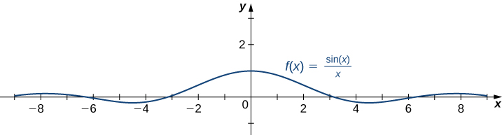

OpenStax, Rice University; Calculus Volume 1. · CC BY-NC-SA 4.0

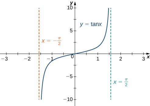
Figure 4.44図 4.44
This function crosses its horizontal asymptote multiple times.
この関数のグラフは、水平漸近線と何度も交わる。
To evaluate $lim_{x \to \infty} {tan}^{−1} (x)$ and $lim_{x \to − \infty} {tan}^{−1} (x),$ we first consider the graph of $y = tan (x)$ over the interval $(− π / 2, π / 2)$ as shown in the following graph.
$lim_{x \to \infty} {tan}^{−1} (x)$ と $lim_{x \to − \infty} {tan}^{−1} (x)$ を求めるため、まず区間 $(− π / 2, π / 2)$ 上の $y = tan (x)$ のグラフを考える。次の図を参照。

OpenStax, Rice University; Calculus Volume 1. · CC BY-NC-SA 4.0

Figure 4.45図 4.45
The graph of $tan x$ has vertical asymptotes at $x = ± \frac{π}{2}$
$tan x$ のグラフは、 $x = ± \frac{π}{2}$ に垂直漸近線をもつ。

Since

まず、次の極限が成り立つ。

lim_{x \to {(π / 2)}^{-}} tan x = \infty,

lim_{x \to {(π / 2)}^{-}} tan x = \infty

it follows that

逆関数の関係から、次式が従う。

lim_{x \to \infty} {tan}^{−1} (x) = \frac{π}{2} .

lim_{x \to \infty} {tan}^{−1} (x) = \frac{π}{2}

Similarly, since

同様に、次の極限も成り立つ。

lim_{x \to {(–π / 2)}^{+}} tan x = − \infty,

lim_{x \to {(–π / 2)}^{+}} tan x = − \infty

it follows that

逆関数の関係から、次式が従う。

lim_{x \to − \infty} {tan}^{−1} (x) = - \frac{π}{2} .

lim_{x \to − \infty} {tan}^{−1} (x) = - \frac{π}{2}

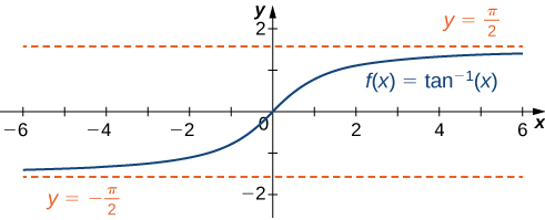
As a result,

y = \frac{π}{2}

and

y = - \frac{π}{2}

are horizontal asymptotes of

f (x) = {tan}^{−1} (x)

as shown in the following graph.

よって、

y = \frac{π}{2}

と

y = - \frac{π}{2}

は

f (x) = {tan}^{−1} (x)

の水平漸近線である。次の図に示す。

f(x)=arctan xのグラフ。左の遠方でy=−π/2へ近づき、原点を通って増加し、右の遠方でy=π/2へ近づく。水平漸近線y=±π/2が破線で描かれている。 — Figure 4.46図 4.46
This function has two horizontal asymptotes.
この関数には二つの水平漸近線がある。

第4章微分の応用

4.6 Limits at Infinity and Asymptotes4.6 無限遠での極限と漸近線

Learning Objectives学習目標

Limits at Infinity無限遠での極限

Limits at Infinity and Horizontal Asymptotes無限遠での極限と水平漸近線

Values of a function f as x→±∞x→±∞のときの関数fの値

Computing Limits at Infinity無限遠での極限を計算する

4.6 Limits at Infinity and Asymptotes4.6　無限遠での極限と漸近線

Values of a function $f$ as $x \to ± \infty$ $x \to ± \infty$ のときの関数 $f$ の値