第4章微分の応用

Differentials微分量

We have seen that linear approximations can be used to estimate function values. They can also be used to estimate the amount a function value changes as a result of a small change in the input. To discuss this more formally, we define a related concept: differentials. Differentials provide us with a way of estimating the amount a function changes as a result of a small change in input values.

英語のヒント

線形近似を使うと、関数の値を近似できることが分かった。さらに、入力のわずかな変化によって関数の値がどれだけ変わるかも近似できる。これをより厳密に述べるために、関連する概念である「微分量」を定義する。微分量は、入力値がわずかに変わったときの、関数の値の変化量を近似する手段となる。

When we first looked at derivatives, we used the Leibniz notation

d y / d x

to represent the derivative of

y

with respect to

x .

Although we used the expressions dy and dx in this notation, they did not have meaning on their own. Here we see a meaning to the expressions dy and dx. Suppose

y = f (x)

is a differentiable function. Let dx be an independent variable that can be assigned any nonzero real number, and define the dependent variable

d y

英語のヒント

微分を初めて扱ったときには、

x

に関する

y

の導関数を表すために、ライプニッツの記法

d y / d x

を使った。この記法に現れるdyとdxには、それぞれ単独での意味をまだ与えていなかった。ここでは、dyとdxという表記に意味を与える。

y = f (x)

を微分可能な関数とする。dxを、0でない任意の実数を割り当てられる独立変数とし、従属変数

d y

を次の式で定義する。

d y = f' (x) d x .

d y = f' (x) d x

(4.2)

It is important to notice that

d y

is a function of both

x

and

d x .

The expressions dy and dx are called differentials. We can divide both sides of Equation 4.2 by

d x,

which yields

d y

が

x

と

d x

の両方の関数であることが重要である。dyとdxを微分量と呼ぶ。式4.2の両辺を

d x

で割ると、次の式が得られる。

\frac{d y}{d x} = f' (x) .

\frac{d y}{d x} = f' (x)

(4.3)

This is the familiar expression we have used to denote a derivative. Equation 4.2 is known as the differential form of Equation 4.3.

これは、導関数を表すために使ってきた見慣れた式である。式4.2は、式4.3の微分形式と呼ばれる。

Example 4.8例題 4.8

Computing differentials微分量を計算する

For each of the following functions, find dy and evaluate when

x = 3

and

d x = 0.1 .

以下の各関数についてdyを求め、

x = 3

、

d x = 0.1

のときの値を計算せよ。

$y = x^{2} + 2 x$
$y = x^{2} + 2 x$
$y = cos x$
$y = cos x$

Solution解き方

The key step is calculating the derivative. When we have that, we can obtain dy directly.

英語のヒント

要となる手順は、導関数を計算することである。それが分かれば、dyはすぐに求められる。

Since $f (x) = x^{2} + 2 x,$ we know $f' (x) = 2 x + 2,$ and therefore
$f (x) = x^{2} + 2 x$ だから、 $f' (x) = 2 x + 2$ である。したがって、

$d y = (2 x + 2) d x .$
$d y = (2 x + 2) d x$

When $x = 3$ and $d x = 0.1,$
$x = 3$ 、 $d x = 0.1$ のとき、

$d y = (2 \cdot 3 + 2) (0.1) = 0.8 .$
$d y = (2 \cdot 3 + 2) (0.1) = 0.8$
Since $f (x) = cos x,$ $f' (x) = − sin (x) .$ This gives us
$f (x) = cos x$ だから、 $f' (x) = − sin (x)$ となる。これより、

$d y = − sin x d x .$
$d y = − sin x d x$

When $x = 3$ and $d x = 0.1,$
$x = 3$ 、 $d x = 0.1$ のとき、

$d y = − sin (3) (0.1) = −0.1 sin (3) .$
$d y = − sin (3) (0.1) = −0.1 sin (3)$

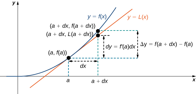
We now connect differentials to linear approximations. Differentials can be used to estimate the change in the value of a function resulting from a small change in input values. Consider a function

f

that is differentiable at point

a .

Suppose the input

x

changes by a small amount. We are interested in how much the output

y

changes. If

x

changes from

a

a + d x,

then the change in

x

d x

(also denoted

Δ x),

and the change in

y

is given by

英語のヒント

次に、微分量と線形近似を結びつけよう。微分量を使うと、入力値が少し変わったことによる、関数の値の変化を近似できる。点

a

で微分可能な関数

f

を考え、入力

x

がわずかに変化するとする。知りたいのは、出力

y

がどれだけ変わるかである。

x

が

a

から

a + d x

に変わるとき、

x

の変化量は

d x

である（別の表記では

Δ x)

。また、

y

の変化量は次のように表せる。

Δ y = f (a + d x) - f (a) .

Δ y = f (a + d x) - f (a)

Instead of calculating the exact change in

y,

however, it is often easier to approximate the change in

y

by using a linear approximation. For

x

near

a,

f (x)

can be approximated by the linear approximation

英語のヒント

しかし、

y

の正確な変化量を計算する代わりに、線形近似で

y

の変化量を近似する方が簡単なことが多い。

x

が

a

に近ければ、

f (x)

を次の一次関数で近似できる。

L (x) = f (a) + f' (a) (x - a) .

L (x) = f (a) + f' (a) (x - a)

Therefore, if

d x

is small,

したがって、

d x

が小さければ、

f (a + d x) \approx L (a + d x) = f (a) + f' (a) (a + d x - a) .

f (a + d x) \approx L (a + d x) = f (a) + f' (a) (a + d x - a)

That is,

すなわち、

f (a + d x) - f (a) \approx L (a + d x) - f (a) = f' (a) d x .

f (a + d x) - f (a) \approx L (a + d x) - f (a) = f' (a) d x

In other words, the actual change in the function

f

x

increases from

a

a + d x

is approximately the difference between

L (a + d x)

and

f (a),

where

L (x)

is the linear approximation of

f

a .

By definition of

L (x),

this difference is equal to

f' (a) d x .

In summary,

英語のヒント

言い換えると、

x

が

a

から

a + d x

に増加したときの、関数

f

の実際の変化量は、

L (a + d x)

と

f (a)

の差にほぼ等しい。ここで、

L (x)

は

a

における

f

の線形近似である。

L (x)

の定義から、この差は

f' (a) d x

に等しい。まとめると、

Δ y = f (a + d x) - f (a) \approx L (a + d x) - f (a) = f' (a) d x = d y .

Δ y = f (a + d x) - f (a) \approx L (a + d x) - f (a) = f' (a) d x = d y

Therefore, we can use the differential

d y = f' (a) d x

to approximate the change in

y

x

increases from

x = a

x = a + d x .

We can see this in the following graph.

したがって、

x

が

x = a

から

x = a + d x

に増加するとき、微分量

d y = f' (a) d x

を使って

y

の変化量を近似できる。この関係を次のグラフに示す。

関数y=f(x)のグラフと、点(a,f(a))での接線L(x)。x軸にはaとa+dxが記され、その間の距離をdxとする破線がある。曲線y=f(x)上に点(a+dx,f(a+dx))、接線y=L(x)上に点(a+dx,L(a+dx))が示されている。f(a)からL(a+dx)までの縦方向の差はdy=f′(a)dx、f(a)からf(a+dx)までの差はΔy=f(a+dx)−f(a)と記されている。 — Figure 4.11図 4.11
The differential $d y = f' (a) d x$ is used to approximate the actual change in $y$ if $x$ increases from $a$ to $a + d x .$
$x$ が $a$ から $a + d x$ に増加するとき、微分量 $d y = f' (a) d x$ を使って $y$ の実際の変化量を近似する。

We now take a look at how to use differentials to approximate the change in the value of the function that results from a small change in the value of the input. Note the calculation with differentials is much simpler than calculating actual values of functions and the result is very close to what we would obtain with the more exact calculation.

英語のヒント

次に、入力の小さな変化によって生じる関数の値の変化を、微分量で近似する方法を見よう。微分量を用いる計算は、関数の値を実際に計算するよりずっと簡単であり、その結果は、より正確な計算で得られる値に非常に近い。

Example 4.9例題 4.9

Approximating Change with Differentials微分量で変化量を近似する

Let

y = x^{2} + 2 x .

Compute

Δ y

and dy at

x = 3

d x = 0.1 .

y = x^{2} + 2 x

とする。

d x = 0.1

のとき、

x = 3

における

Δ y

とdyを求めよ。

Solution解き方

The actual change in

y

x

changes from

x = 3

x = 3.1

is given by

x

が

x = 3

から

x = 3.1

に変化するとき、

y

の実際の変化量は、

Δ y = f (3.1) - f (3) = [{(3.1)}^{2} + 2 (3.1)] - [3^{2} + 2 (3)] = 0.81 .

Δ y = f (3.1) - f (3) = [{(3.1)}^{2} + 2 (3.1)] - [3^{2} + 2 (3)] = 0.81

The approximate change in

y

is given by

d y = f' (3) d x .

Since

f' (x) = 2 x + 2,

we have

y

の変化量の近似は

d y = f' (3) d x

で与えられる。

f' (x) = 2 x + 2

なので、

d y = f' (3) d x = (2 (3) + 2) (0.1) = 0.8 .

d y = f' (3) d x = (2 (3) + 2) (0.1) = 0.8

Calculating the Amount of Error誤差の大きさを計算する

Any type of measurement is prone to a certain amount of error. In many applications, certain quantities are calculated based on measurements. For example, the area of a circle is calculated by measuring the radius of the circle. An error in the measurement of the radius leads to an error in the computed value of the area. Here we examine this type of error and study how differentials can be used to estimate the error.

英語のヒント

どのような測定にも、ある程度の誤差が生じる。応用の多くでは、測定した値を使って別の量を計算する。例えば円の面積は、半径を測定して計算する。半径の測定に誤差があれば、計算で求めた面積にも誤差が生じる。ここでは、この種の誤差を調べ、微分量を使って誤差を見積もる方法を学ぶ。

Consider a function

f

with an input that is a measured quantity. Suppose the exact value of the measured quantity is

a,

but the measured value is

a + d x .

We say the measurement error is dx (or

Δ x) .

As a result, an error occurs in the calculated quantity

f (x) .

This type of error is known as a propagated error and is given by

英語のヒント

測定された量を入力とする関数

f

を考える。その量の真の値を

a

、測定値を

a + d x

とする。このとき、測定誤差はdx（別の表記では

Δ x)

である。その結果、計算で求める量

f (x)

にも誤差が生じる。この誤差を伝播誤差と呼び、次の式で表す。

Δ y = f (a + d x) - f (a) .

Δ y = f (a + d x) - f (a)

Since all measurements are prone to some degree of error, we do not know the exact value of a measured quantity, so we cannot calculate the propagated error exactly. However, given an estimate of the accuracy of a measurement, we can use differentials to approximate the propagated error

Δ y .

Specifically, if

f

is a differentiable function at

a,

the propagated error is

英語のヒント

測定には必ずある程度の誤差があるため、測定した量の真の値は分からず、伝播誤差を厳密に計算することはできない。しかし、測定の精度を見積もれるなら、微分量を使って伝播誤差

Δ y

を近似できる。具体的には、

f

が

a

で微分可能なら、伝播誤差は次のようになる。

Δ y \approx d y = f' (a) d x .

Δ y \approx d y = f' (a) d x

Unfortunately, we do not know the exact value

a .

However, we can use the measured value

a + d x,

and estimate

ただし、真の値

a

は分からない。そこで測定値

a + d x

を使い、次のように見積もることができる。

Δ y \approx d y \approx f' (a + d x) d x .

Δ y \approx d y \approx f' (a + d x) d x

In the next example, we look at how differentials can be used to estimate the error in calculating the volume of a box if we assume the measurement of the side length is made with a certain amount of accuracy.

英語のヒント

次の例では、一辺の長さがある精度で測定されていると仮定して、箱の体積の計算に生じる誤差を微分量で見積もる方法を調べる。

Example 4.10例題 4.10

Volume of a Cube立方体の体積

Suppose the side length of a cube is measured to be 5 cm with an accuracy of 0.1 cm.

立方体の一辺の長さを測定したところ、0.1 cmの精度で5 cmであったとする。

Use differentials to estimate the error in the computed volume of the cube.
微分量を使って、計算で求めた立方体の体積の誤差を見積もれ。
Compute the volume of the cube if the side length is (i) 4.9 cm and (ii) 5.1 cm to compare the estimated error with the actual potential error.
一辺が(i) 4.9 cmの場合と(ii) 5.1 cmの場合の体積を計算し、見積もった誤差と、実際に生じ得る誤差を比較せよ。

Solution解き方

The measurement of the side length is accurate to within $± 0.1$ cm. Therefore,
一辺の測定値の誤差は $± 0.1$ cm以内である。したがって、

$−0.1 \leq d x \leq 0.1 .$
$−0.1 \leq d x \leq 0.1$

The volume of a cube is given by $V = x^{3},$ which leads to
立方体の体積は $V = x^{3}$ なので、

$d V = 3 x^{2} d x .$
$d V = 3 x^{2} d x$

Using the measured side length of 5 cm, we can estimate that
測定した一辺の長さ5 cmを使うと、次のように見積もれる。

$−3 {(5)}^{2} (0.1) \leq d V \leq 3 {(5)}^{2} (0.1) .$
$−3 {(5)}^{2} (0.1) \leq d V \leq 3 {(5)}^{2} (0.1)$

Therefore,
したがって、

$−7.5 \leq d V \leq 7.5 .$
$−7.5 \leq d V \leq 7.5$
If the side length is actually 4.9 cm, then the volume of the cube is
一辺の実際の長さが4.9 cmなら、立方体の体積は、

$V (4.9) = {(4.9)}^{3} = 117.649 {cm}^{3} .$
$V (4.9) = {(4.9)}^{3} = 117.649 {cm}^{3}$

If the side length is actually 5.1 cm, then the volume of the cube is
一辺の実際の長さが5.1 cmなら、立方体の体積は、

$V (5.1) = {(5.1)}^{3} = 132.651 {cm}^{3} .$
$V (5.1) = {(5.1)}^{3} = 132.651 {cm}^{3}$

Therefore, the actual volume of the cube is between 117.649 and 132.651. Since the side length is measured to be 5 cm, the computed volume is $V (5) = 5^{3} = 125 .$ Therefore, the error in the computed volume is
したがって、実際の体積は117.649から132.651の間にある。一辺の測定値は5 cmなので、計算で得られる体積は $V (5) = 5^{3} = 125$ である。そのため、この体積の計算値の誤差は、

$117.649 - 125 \leq Δ V \leq 132.651 - 125 .$
$117.649 - 125 \leq Δ V \leq 132.651 - 125$

That is,
すなわち、

$−7.351 \leq Δ V \leq 7.651 .$
$−7.351 \leq Δ V \leq 7.651$

We see the estimated error $d V$ is relatively close to the actual potential error in the computed volume.
見積もった誤差 $d V$ は、体積の計算値に実際に生じ得る誤差に比較的近いことが分かる。

The measurement error dx

(=Δ x)

and the propagated error

Δ y

are absolute errors. We are typically interested in the size of an error relative to the size of the quantity being measured or calculated. Given an absolute error

Δ q

for a particular quantity, we define the relative error as

\frac{Δ q}{q},

where

q

is the actual value of the quantity. The percentage error is the relative error expressed as a percentage. For example, if we measure the height of a ladder to be 63 in. when the actual height is 62 in., the absolute error is 1 in. but the relative error is

\frac{1}{62} = 0.016,

1.6 % .

By comparison, if we measure the width of a piece of cardboard to be 8.25 in. when the actual width is 8 in., our absolute error is

\frac{1}{4}

in., whereas the relative error is

\frac{0.25}{8} = \frac{1}{32},

3.1 % .

Therefore, the percentage error in the measurement of the cardboard is larger, even though 0.25 in. is less than 1 in.

英語のヒント

測定誤差dx

(=Δ x)

と伝播誤差

Δ y

は、絶対誤差である。通常は、誤差そのものの大きさに加えて、測定・計算する量に対して誤差がどの程度の割合なのかに関心がある。ある量の絶対誤差が

Δ q

であるとき、相対誤差を

\frac{Δ q}{q}

と定義する。ここで、

q

はその量の真の値である。百分率誤差とは、この相対誤差を百分率で表したものをいう。例えば、実際には62 in.のはしごの高さを63 in.と測定したなら、絶対誤差は1 in.だが、相対誤差は

\frac{1}{62} = 0.016

、すなわち

1.6 %

となる。一方、実際には8 in.の厚紙の幅を8.25 in.と測定した場合、絶対誤差は

\frac{1}{4}

in.、相対誤差は

\frac{0.25}{8} = \frac{1}{32}

、すなわち

3.1 %

である。したがって、0.25 in.は1 in.より小さくても、厚紙の測定の方が百分率誤差は大きい。

Example 4.11例題 4.11

Relative and Percentage Error相対誤差と百分率誤差

An astronaut using a camera measures the radius of Earth as 4000 mi with an error of

± 80

mi. Let’s use differentials to estimate the relative and percentage error of using this radius measurement to calculate the volume of Earth, assuming the planet is a perfect sphere.

英語のヒント

宇宙飛行士がカメラを使い、地球の半径を誤差

± 80

miで4000 miと測定した。この半径の測定値から地球の体積を計算するときの相対誤差と百分率誤差を、微分量で見積もろう。地球は完全な球だと仮定する。

Solution解き方

If the measurement of the radius is accurate to within

± 80,

we have

半径の測定誤差が

± 80

以内であるなら、

−80 \leq d r \leq 80 .

−80 \leq d r \leq 80

Since the volume of a sphere is given by

V = (\frac{4}{3}) π r^{3},

we have

球の体積は

V = (\frac{4}{3}) π r^{3}

で与えられるので、

d V = 4 π r^{2} d r .

d V = 4 π r^{2} d r

Using the measured radius of 4000 mi, we can estimate

測定した半径4000 miを使うと、次のように見積もれる。

−4 π {(4000)}^{2} (80) \leq d V \leq 4 π {(4000)}^{2} (80) .

−4 π {(4000)}^{2} (80) \leq d V \leq 4 π {(4000)}^{2} (80)

To estimate the relative error, consider

\frac{d V}{V} .

Since we do not know the exact value of the volume

V,

use the measured radius

r = 4000 mi

to estimate

V .

We obtain

V \approx (\frac{4}{3}) π {(4000)}^{3} .

Therefore the relative error satisfies

相対誤差の見積もりには

\frac{d V}{V}

を考える。体積

V

の真の値は分からないので、測定した半径

r = 4000 mi

を使って

V

を近似する。すると

V \approx (\frac{4}{3}) π {(4000)}^{3}

となる。したがって、相対誤差の見積もりは次の関係を満たす。

\frac{−4 π {(4000)}^{2} (80)}{4 π {(4000)}^{3} / 3} \leq \frac{d V}{V} \leq \frac{4 π {(4000)}^{2} (80)}{4 π {(4000)}^{3} / 3},

\frac{−4 π {(4000)}^{2} (80)}{4 π {(4000)}^{3} / 3} \leq \frac{d V}{V} \leq \frac{4 π {(4000)}^{2} (80)}{4 π {(4000)}^{3} / 3}

which simplifies to

整理すると、

−0.06 \leq \frac{d V}{V} \leq 0.06 .

−0.06 \leq \frac{d V}{V} \leq 0.06

The relative error is 0.06 and the percentage error is

6 % .

相対誤差は0.06、百分率誤差は

6 %

と見積もられる。