第2章記述統計

2.2 Histograms, Frequency Polygons, and Time Series Graphs2.2　ヒストグラム、度数折れ線、時系列グラフ

For most of the work you do in this book, you will use a histogram to display the data. One advantage of a histogram is that it can readily display large data sets. A rule of thumb is to use a histogram when the data set consists of 100 values or more.

英語のヒント

本書で行う作業の多くでは、データの表示にヒストグラムを使う。大規模なデータセットを容易に示せることが、その利点の1つである。目安として、データの値が100個以上あればヒストグラムを用いる。

A histogram consists of contiguous (adjoining) boxes. It has both a horizontal axis and a vertical axis. The horizontal axis is labeled with what the data represents (for instance, distance from your home to school). The vertical axis is labeled either frequency or relative frequency (or percent frequency or probability). The graph will have the same shape with either label. The histogram (like the stemplot) can give you the shape of the data, the center, and the spread of the data.

英語のヒント

ヒストグラムは、互いに接する長方形からなる。横軸と縦軸を持ち、横軸にはデータが表すもの（例えば自宅から学校までの距離）を示す。縦軸には度数か相対度数（あるいは百分率度数や確率）を示す。どちらでもグラフの形は同じになる。幹葉図と同じく、ヒストグラムからデータの形、中心、散らばりが分かる。

The relative frequency is equal to the frequency for an observed value of the data divided by the total number of data values in the sample. (Remember, frequency is defined as the number of times an answer occurs.) If:

相対度数は、観測されたデータの値の度数を、標本のデータ総数で割ったものである。（度数は、ある回答が現れる回数と定義されることを思い出そう。）次のように置くと、

f = frequency
f＝度数
n = total number of data values (or the sum of the individual frequencies), and
n＝データの総数（または個々の度数の合計）
RF = relative frequency,
RF＝相対度数

then:

次の式が成り立つ。

RF = \frac{f}{n}

For example, if three students in an English class of 40 students received from 90% to 100%, then, f = 3, n = 40, and RF =

\frac{f}{n}

\frac{3}{40}

= 0.075. 7.5% of the students received 90–100%. 90–100% are quantitative measures.

例えば、40人の英語のクラスで、3人の得点率が90～100％だったなら、f＝3、n＝40、RF＝

\frac{f}{n}

＝

\frac{3}{40}

＝0.075となる。学生の7.5％が90～100％を得た。90～100％は量的な測定値である。

To construct a histogram, first decide how many bars or intervals, also called classes, represent the data. Many histograms consist of five to 15 bars or classes for clarity. The number of bars needs to be chosen. Choose a starting point for the first interval to be less than the smallest data value. A convenient starting point is a lower value carried out to one more decimal place than the value with the most decimal places. For example, if the value with the most decimal places is 6.1 and this is the smallest value, a convenient starting point is 6.05 (6.1 – 0.05 = 6.05). We say that 6.05 has more precision. If the value with the most decimal places is 2.23 and the lowest value is 1.5, a convenient starting point is 1.495 (1.5 – 0.005 = 1.495). If the value with the most decimal places is 3.234 and the lowest value is 1.0, a convenient starting point is 0.9995 (1.0 – 0.0005 = 0.9995). If all the data happen to be integers and the smallest value is two, then a convenient starting point is 1.5 (2 – 0.5 = 1.5). Also, when the starting point and other boundaries are carried to one additional decimal place, no data value will fall on a boundary. The next two examples go into detail about how to construct a histogram using continuous data and how to create a histogram using discrete data.

英語のヒント

ヒストグラムを作るには、まず、データをいくつの棒、つまり区間（階級ともいう）で表すかを決める。見やすさのため、5～15本の棒または階級で構成することが多い。棒の本数は自分で選ぶ必要がある。最初の区間の始点は、最小のデータより小さくする。小数点以下の桁数が最も多い値より、さらに1桁多く取った小さな値が便利である。例えば、桁数が最も多い値が6.1で、これが最小値でもあるなら、始点は6.05とするとよい（6.1−0.05＝6.05）。6.05は精度が高いという。桁数が最も多い値が2.23で、最小値が1.5なら、始点は1.495が便利である（1.5−0.005＝1.495）。桁数が最も多い値が3.234で、最小値が1.0なら、0.9995を始点にできる（1.0−0.0005＝0.9995）。すべて整数で最小値が2なら、始点は1.5が便利である（2−0.5＝1.5）。始点やほかの境界値を1桁細かく設定すると、データの値が境界上に来なくなる。続く2つの例では、連続データと離散データを使ったヒストグラムの作成を詳しく説明する。

Example 2.7例題 2.7

The following data are the heights (in inches to the nearest half inch) of 100 semiprofessional soccer players. The heights are continuous data, since height is measured.
60; 60.5; 61; 61; 61.5
63.5; 63.5; 63.5
64; 64; 64; 64; 64; 64; 64; 64.5; 64.5; 64.5; 64.5; 64.5; 64.5; 64.5; 64.5
66; 66; 66; 66; 66; 66; 66; 66; 66; 66; 66.5; 66.5; 66.5; 66.5; 66.5; 66.5; 66.5; 66.5; 66.5; 66.5; 66.5; 67; 67; 67; 67; 67; 67; 67; 67; 67; 67; 67; 67; 67.5; 67.5; 67.5; 67.5; 67.5; 67.5; 67.5
68; 68; 69; 69; 69; 69; 69; 69; 69; 69; 69; 69; 69.5; 69.5; 69.5; 69.5; 69.5
70; 70; 70; 70; 70; 70; 70.5; 70.5; 70.5; 71; 71; 71
72; 72; 72; 72.5; 72.5; 73; 73.5
74

以下は、セミプロのサッカー選手100人の身長を、最も近い0.5インチ単位まで測定したデータである。身長は測定する量なので、連続データである。60; 60.5; 61; 61; 61.5 63.5; 63.5; 63.5 64; 64; 64; 64; 64; 64; 64; 64.5; 64.5; 64.5; 64.5; 64.5; 64.5; 64.5; 64.5 66; 66; 66; 66; 66; 66; 66; 66; 66; 66; 66.5; 66.5; 66.5; 66.5; 66.5; 66.5; 66.5; 66.5; 66.5; 66.5; 66.5; 67; 67; 67; 67; 67; 67; 67; 67; 67; 67; 67; 67; 67.5; 67.5; 67.5; 67.5; 67.5; 67.5; 67.5 68; 68; 69; 69; 69; 69; 69; 69; 69; 69; 69; 69; 69.5; 69.5; 69.5; 69.5; 69.5 70; 70; 70; 70; 70; 70; 70.5; 70.5; 70.5; 71; 71; 71 72; 72; 72; 72.5; 72.5; 73; 73.5 74

The smallest data value is 60. Since the data with the most decimal places has one decimal (for instance, 61.5), we want our starting point to have two decimal places. Since the numbers 0.5, 0.05, 0.005, etc. are convenient numbers, use 0.05 and subtract it from 60, the smallest value, for the convenient starting point.

最小のデータは60である。小数点以下の桁数が最も多いデータでも1桁（例えば61.5）なので、始点は小数第2位まで取る。0.5、0.05、0.005などは扱いやすい数であるため、0.05を使い、最小値60から引いて始点とする。

60 – 0.05 = 59.95 which is more precise than, say, 61.5 by one decimal place. The starting point is, then, 59.95.

60−0.05＝59.95は、例えば61.5より小数点以下が1桁細かい。したがって、始点は59.95となる。

The largest value is 74, so 74 + 0.05 = 74.05 is the ending value.

最大値は74なので、終点は74＋0.05＝74.05となる。

Next, calculate the width of each bar or class interval. To calculate this width, subtract the starting point from the ending value and divide by the number of bars (you must choose the number of bars you desire). Suppose you choose eight bars.

次に、各棒、つまり階級区間の幅を計算する。終点から始点を引き、棒の本数で割る（本数は自分で決める）。ここでは8本にするとしよう。

\begin{matrix} 74.05 - 59.95 = 14.1 \\ 14.1 \div 8 = 1.76 \end{matrix}

NOTE注

We will round up to two and make each bar or class interval two units wide. Rounding up to two is one way to prevent a value from falling on a boundary. Rounding to the next number is often necessary even if it goes against the standard rules of rounding. For this example, using 1.76 as the width would also work. A guideline that is followed by some for the number of bars or class intervals is to take the square root of the number of data values and then round to the nearest whole number, if necessary. For example, if there are 150 values of data, take the square root of 150 and round to 12 bars or intervals.

値を2に切り上げ、各棒、つまり階級区間の幅を2とする。2への切り上げは、データの値が境界上に来るのを防ぐ方法の1つである。通常の丸め方に反していても、次の数に切り上げる必要が生じることは多い。この例では、幅を1.76としてもよい。棒または階級区間の数を決める目安として、データ数の平方根を取り、必要なら最も近い整数に丸める方法もある。例えばデータが150個なら、150の平方根を丸め、12本の棒または区間とする。

The boundaries are:

境界値は以下のとおりである。

59.95
59.95 + 2 = 61.95
61.95 + 2 = 63.95
63.95 + 2 = 65.95
65.95 + 2 = 67.95
67.95 + 2 = 69.95
69.95 + 2 = 71.95
71.95 + 2 = 73.95
73.95 + 2 = 75.95

The heights 60 through 61.5 inches are in the interval 59.95–61.95. The heights that are 63.5 are in the interval 61.95–63.95. The heights that are 64 through 64.5 are in the interval 63.95–65.95. The heights 66 through 67.5 are in the interval 65.95–67.95. The heights 68 through 69.5 are in the interval 67.95–69.95. The heights 70 through 71 are in the interval 69.95–71.95. The heights 72 through 73.5 are in the interval 71.95–73.95. The height 74 is in the interval 73.95–75.95.

60～61.5インチの身長は、区間59.95～61.95に入る。63.5インチは61.95～63.95に、64～64.5インチは63.95～65.95に入る。66～67.5インチは65.95～67.95に入る。68～69.5インチは67.95～69.95に、70～71インチは69.95～71.95に、72～73.5インチは71.95～73.95に入る。74インチは73.95～75.95に入る。

The following histogram displays the heights on the x-axis and relative frequency on the y-axis.

以下のヒストグラムは、x軸に身長、y軸に相対度数を示す。

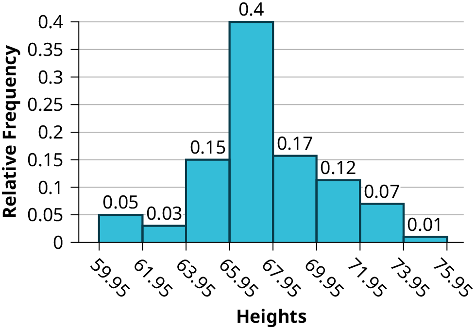
8本の棒からなるヒストグラム。縦軸は0～0.4を0.05刻み、横軸は59.95～75.95を2刻みで示す。 — Figure 2.12図 2.12

Try Itやってみよう

The following data are the shoe sizes of 50 students. The sizes are discrete data since shoe size is measured in whole and half units only. Construct a histogram and calculate the width of each bar or class interval. Suppose you choose six bars.
9; 9; 9.5; 9.5; 10; 10; 10; 10; 10; 10; 10.5; 10.5; 10.5; 10.5; 10.5; 10.5; 10.5; 10.5
11; 11; 11; 11; 11; 11; 11; 11; 11; 11; 11; 11; 11; 11.5; 11.5; 11.5; 11.5; 11.5; 11.5; 11.5
12; 12; 12; 12; 12; 12; 12; 12.5; 12.5; 12.5; 12.5; 14

以下は学生50人の靴のサイズのデータである。靴のサイズは整数またはその中間の0.5単位でしか測らないため、離散データである。ヒストグラムを作成し、各棒、つまり階級区間の幅を計算せよ。棒は6本とする。9; 9; 9.5; 9.5; 10; 10; 10; 10; 10; 10; 10.5; 10.5; 10.5; 10.5; 10.5; 10.5; 10.5; 10.5 11; 11; 11; 11; 11; 11; 11; 11; 11; 11; 11; 11; 11; 11.5; 11.5; 11.5; 11.5; 11.5; 11.5; 11.5 12; 12; 12; 12; 12; 12; 12; 12.5; 12.5; 12.5; 12.5; 14

Example 2.8例題 2.8

Create a histogram for the following data: the number of books bought by 50 part-time college students at ABC College. The number of books is discrete data, since books are counted.
1; 1; 1; 1; 1; 1; 1; 1; 1; 1; 1
2; 2; 2; 2; 2; 2; 2; 2; 2; 2
3; 3; 3; 3; 3; 3; 3; 3; 3; 3; 3; 3; 3; 3; 3; 3
4; 4; 4; 4; 4; 4
5; 5; 5; 5; 5
6; 6

ABC大学のパートタイム学生50人が購入した本の冊数について、ヒストグラムを作成せよ。本は数えるものなので、冊数は離散データである。1; 1; 1; 1; 1; 1; 1; 1; 1; 1; 1 2; 2; 2; 2; 2; 2; 2; 2; 2; 2 3; 3; 3; 3; 3; 3; 3; 3; 3; 3; 3; 3; 3; 3; 3; 3 4; 4; 4; 4; 4; 4 5; 5; 5; 5; 5 6; 6

Eleven students buy one book. Ten students buy two books. Sixteen students buy three books. Six students buy four books. Five students buy five books. Two students buy six books.

1冊買う学生は11人、2冊は10人、3冊は16人、4冊は6人、5冊は5人、6冊は2人である。

Because the data are integers, subtract 0.5 from 1, the smallest data value and add 0.5 to 6, the largest data value. Then the starting point is 0.5 and the ending value is 6.5.

データは整数なので、最小値1から0.5を引き、最大値6に0.5を足す。すると始点は0.5、終点は6.5となる。

Next, calculate the width of each bar or class interval. If the data are discrete and there are not too many different values, a width that places the data values in the middle of the bar or class interval is the most convenient. Since the data consist of the numbers 1, 2, 3, 4, 5, 6, and the starting point is 0.5, a width of one places the 1 in the middle of the interval from 0.5 to 1.5, the 2 in the middle of the interval from 1.5 to 2.5, the 3 in the middle of the interval from 2.5 to 3.5, the 4 in the middle of the interval from _______ to _______, the 5 in the middle of the interval from _______ to _______, and the _______ in the middle of the interval from _______ to _______ .

次に、各棒、つまり階級区間の幅を計算する。離散データで値の種類が多すぎない場合、値が棒や階級区間の中央に来るような幅が最も便利である。データは1、2、3、4、5、6で、始点は0.5である。幅を1にすると、1は区間0.5～1.5の中央、2は1.5～2.5の中央、3は2.5～3.5の中央に来る。4は_______～_______の中央、5は_______～_______の中央、_______は_______～_______の中央に来る。

Solution解き方

3.5 to 4.5
3.5～4.5
4.5 to 5.5
4.5～5.5
6
5.5 to 6.5
5.5～6.5

Calculate the number of bars as follows:

棒の本数を次のように計算する。

\begin{matrix} 6.5 - 0.5 = 6 \\ 6 \div 1 = 6 \end{matrix}

where 1 is the width of a bar. Therefore, bars = 6.

ここで1は棒の幅である。したがって、棒は6本となる。

The following histogram displays the number of books on the x-axis and the frequency on the y-axis.

以下のヒストグラムは、x軸に本の冊数、y軸に度数を示す。

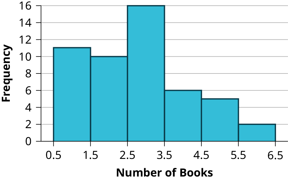
6本の棒からなるヒストグラム。縦軸は0～16を2刻み、横軸は0.5～6.5を1刻みで示す。 — Figure 2.13図 2.13

Using the Calculator電卓の操作

Go to NOTEs for the TI-83, 83+, 84, 84+ Calculators. There are calculator instructions for entering data and for creating a customized histogram. Create the histogram for Example 2.8.

「TI-83、83+、84、84+電卓の操作メモ」を参照せよ。データを入力し、設定を調整したヒストグラムを作る手順が載っている。例題2.8のヒストグラムを作成せよ。

Press Y=. Press CLEAR to delete any equations.
Y=を押し、CLEARで式を削除する。
Press STAT 1:EDIT. If L1 has data in it, arrow up into the name L1, press CLEAR and then arrow down. If necessary, do the same for L2.
STATの1:EDITを選ぶ。L1にデータがあれば、上矢印キーでL1という名前へ移動し、CLEARを押してから下矢印キーを押す。必要ならL2でも同様に行う。
Into L1, enter 1, 2, 3, 4, 5, 6.
L1に1, 2, 3, 4, 5, 6と入力する。
Into L2, enter 11, 10, 16, 6, 5, 2.
L2に11, 10, 16, 6, 5, 2と入力する。
Press WINDOW. Set Xmin = .5, Xmax = 6.5, Xscl = (6.5 – .5)/6, Ymin = –1, Ymax = 20, Yscl = 1, Xres = 1.
WINDOWを押し、Xmin＝.5、Xmax＝6.5、Xscl＝(6.5−.5)/6、Ymin＝−1、Ymax＝20、Yscl＝1、Xres＝1と設定する。
Press 2^nd Y=. Start by pressing 4:Plotsoff ENTER.
2^nd、Y=を押す。まず4:Plotsoff、ENTERと押す。
Press 2^nd Y=. Press 1:Plot1. Press ENTER. Arrow down to TYPE. Arrow to the 3^rd picture (histogram). Press ENTER.
2^nd、Y=を押し、1:Plot1を選んでENTERを押す。下矢印キーでTYPEへ移動し、3番目の図（ヒストグラム）を選んでENTERを押す。
Arrow down to Xlist: Enter L1 (2^nd 1). Arrow down to Freq. Enter L2 (2^nd 2).
下矢印キーでXlistへ移動し、L1（2^nd、1）と入力する。下矢印キーでFreqへ移動し、L2（2^nd、2）と入力する。
Press GRAPH.
GRAPHを押す。
Use the TRACE key and the arrow keys to examine the histogram.
TRACEキーと矢印キーでヒストグラムを調べる。

Try Itやってみよう

The following data are the number of sports played by 50 student athletes. The number of sports is discrete data since sports are counted.

以下のデータは、学生選手50人が行うスポーツの種目数である。種目は数えるものなので、種目数は離散データである。

1; 1; 1; 1; 1; 1; 1; 1; 1; 1; 1; 1; 1; 1; 1; 1; 1; 1; 1; 1
2; 2; 2; 2; 2; 2; 2; 2; 2; 2; 2; 2; 2; 2; 2; 2; 2; 2; 2; 2; 2; 2
3; 3; 3; 3; 3; 3; 3; 3
20 student athletes play one sport. 22 student athletes play two sports. Eight student athletes play three sports.

1; 1; 1; 1; 1; 1; 1; 1; 1; 1; 1; 1; 1; 1; 1; 1; 1; 1; 1; 1 2; 2; 2; 2; 2; 2; 2; 2; 2; 2; 2; 2; 2; 2; 2; 2; 2; 2; 2; 2; 2; 2 3; 3; 3; 3; 3; 3; 3; 3学生選手の20人は1種目、22人は2種目、8人は3種目を行っている。

Fill in the blanks for the following sentence. Since the data consist of the numbers 1, 2, 3, and the starting point is 0.5, a width of one places the 1 in the middle of the interval 0.5 to _____, the 2 in the middle of the interval from _____ to _____, and the 3 in the middle of the interval from _____ to _____.

次の文の空欄を埋めよ。データは1、2、3で、始点は0.5である。幅を1にすると、1は区間0.5～_____の中央、2は_____～_____の中央、3は_____～_____の中央に来る。

Example 2.9例題 2.9

Using this data set, construct a histogram.

このデータセットでヒストグラムを作成せよ。

Table 2.21表 2.21
Number of Hours My Classmates Spent Playing Video Games on Weekends クラスの学生が週末にビデオゲームに費やした時間
9.95	10	2.25	16.75	0
19.5	22.5	7.5	15	12.75
5.5	11	10	20.75	17.5
23	21.9	24	23.75	18
20	15	22.9	18.8	20.5

Solution解き方

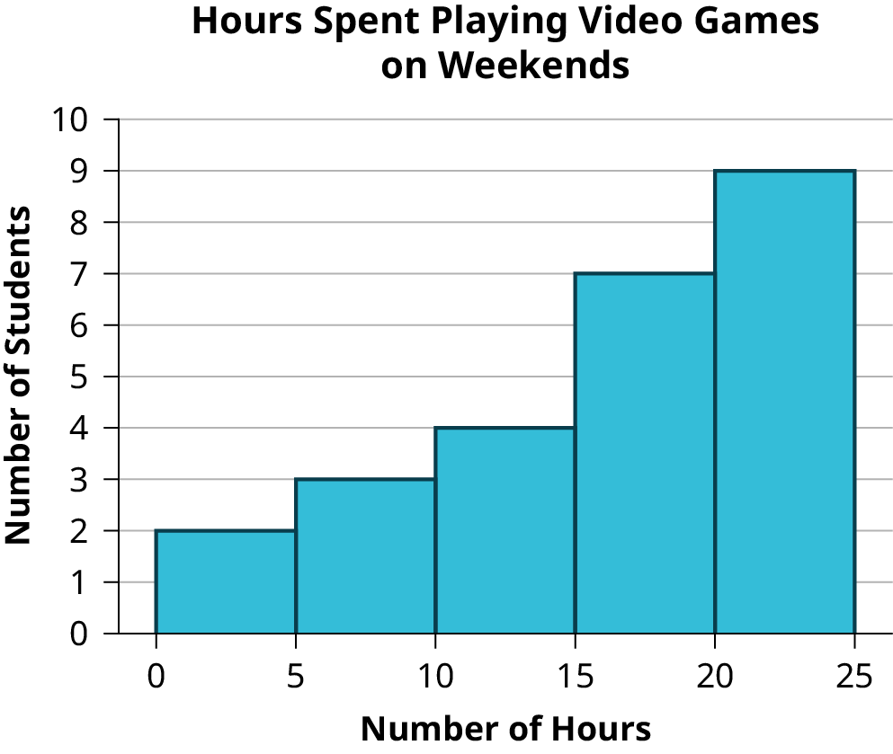
与えられたデータに対応するヒストグラム。横軸は0～25を幅5の5本の棒に分け、縦軸は0～10を1刻みで示す。横軸は週末にビデオゲームに費やした時間、縦軸は学生数である。 — Figure 2.14図 2.14

Some values in this data set fall on boundaries for the class intervals. A value is counted in a class interval if it falls on the left boundary, but not if it falls on the right boundary. Different researchers may set up histograms for the same data in different ways. There is more than one correct way to set up a histogram.

このデータセットには、階級区間の境界上に来る値がある。左側の境界上の値はその区間に含め、右側の境界上の値は含めない。同じデータでも、研究者によって異なるヒストグラムを作ることがある。正しい作り方は1つとは限らない。

Collaborative Exercise共同演習

第2章記述統計

2.2 Histograms, Frequency Polygons, and Time Series Graphs2.2 ヒストグラム、度数折れ線、時系列グラフ

2.2 Histograms, Frequency Polygons, and Time Series Graphs2.2　ヒストグラム、度数折れ線、時系列グラフ