第2章記述統計

2.1 Stem-and-Leaf Graphs (Stemplots), Line Graphs, and Bar Graphs2.1　幹葉図、折れ線グラフ、棒グラフ

One simple graph, the stem-and-leaf graph or stemplot, comes from the field of exploratory data analysis. It is a good choice when the data sets are small. To create the plot, divide each observation of data into a stem and a leaf. The leaf consists of a final significant digit. For example, 23 has stem two and leaf three. The number 432 has stem 43 and leaf two. Likewise, the number 5,432 has stem 543 and leaf two. The decimal 9.3 has stem nine and leaf three. Write the stems in a vertical line from smallest to largest. Draw a vertical line to the right of the stems. Then write the leaves in increasing order next to their corresponding stem.

英語のヒント

単純なグラフの1つである幹葉図は、探索的データ分析の分野から生まれた。データセットが小さい場合に適している。作成するには、各観測値を「幹」と「葉」に分ける。葉は、最後の有効な1桁である。例えば、23なら幹は2、葉は3となる。432なら幹は43、葉は2である。同様に、5,432なら幹は543、葉は2である。小数9.3なら幹は9、葉は3である。幹を小さい順に縦に並べ、その右側に縦線を引く。次に、対応する幹の横に、葉を小さい順に書き込む。

Example 2.1例題 2.1

For Professor Dean's spring pre-calculus class, scores for the first exam were as follows (smallest to largest):
33; 42; 49; 49; 53; 55; 55; 61; 63; 67; 68; 68; 69; 69; 72; 73; 74; 78; 80; 83; 88; 88; 88; 90; 92; 94; 94; 94; 94; 96; 100

ディーン教授の春学期の微積分準備の授業で、最初の試験の点数は次のとおりだった（小さい順）。33; 42; 49; 49; 53; 55; 55; 61; 63; 67; 68; 68; 69; 69; 72; 73; 74; 78; 80; 83; 88; 88; 88; 90; 92; 94; 94; 94; 94; 96; 100

Stem-and-Leaf Graph幹葉図

Table 2.1表 2.1
Stem 幹	Leaf 葉
3	3
4	2 9 9
5	3 5 5
6	1 3 7 8 8 9 9
7	2 3 4 8
8	0 3 8 8 8
9	0 2 4 4 4 4 6
10	0

The stemplot shows that most scores fell in the 60s, 70s, 80s, and 90s. Eight out of the 31 scores or approximately 26%

(\frac{8}{31})

were in the 90s or 100, a fairly high number of As.

幹葉図から、点数の大部分が60点台、70点台、80点台、90点台だったと分かる。31人中8人、つまり約26％

(\frac{8}{31})

が90点台か100点であり、A評価がかなり多い。

The stemplot is a quick way to graph data and gives an exact picture of the data. You want to look for an overall pattern and any outliers. An outlier is an observation of data that does not fit the rest of the data. It is sometimes called an extreme value. When you graph an outlier, it will appear not to fit the pattern of the graph. Some outliers are due to mistakes (for example, writing down 50 instead of 500) while others may indicate that something unusual is happening. It takes some background information to explain outliers, so we will cover them in more detail later.

英語のヒント

幹葉図は、すばやくデータを図示し、その正確な姿を示す方法である。全体的なパターンと外れ値に着目する。外れ値とは、ほかのデータになじまない観測値であり、極端値ともいう。外れ値を図にすると、そのグラフのパターンから外れて見える。500と書くべきところを50と書くような間違いによる外れ値もあれば、何か異常が起きていることを示す外れ値もある。外れ値の説明には背景情報が必要なので、後で詳しく扱う。

Example 2.2例題 2.2

The data are the distances (in kilometers) from a home to local supermarkets. Create a stemplot using the data:
1.1; 1.5; 2.3; 2.5; 2.7; 3.2; 3.3; 3.3; 3.5; 3.8; 4.0; 4.2; 4.5; 4.5; 4.7; 4.8; 5.5; 5.6; 6.5; 6.7; 12.3

データは、ある家から近隣のスーパーまでの距離（キロメートル）である。次のデータで幹葉図を作成せよ。1.1; 1.5; 2.3; 2.5; 2.7; 3.2; 3.3; 3.3; 3.5; 3.8; 4.0; 4.2; 4.5; 4.5; 4.7; 4.8; 5.5; 5.6; 6.5; 6.7; 12.3

Do the data seem to have any concentration of values?

値が集中しているところはありそうか。

Solution解き方

The value 12.3 may be an outlier. Values appear to concentrate at three and four kilometers.

12.3は外れ値かもしれない。値は3～4キロメートル付近に集中しているようである。

Table 2.2表 2.2
Stem 幹	Leaf 葉
1	1 5
2	3 5 7
3	2 3 3 5 8
4	0 2 5 5 7 8
5	5 6
6	5 7
7
8
9
10
11
12	3

Example 2.3例題 2.3

A side-by-side stem-and-leaf plot allows a comparison of the two data sets in two columns. In a side-by-side stem-and-leaf plot, two sets of leaves share the same stem. The leaves are to the left and the right of the stems. Table 2.3 and Table 2.4 show the ages of presidents at their inauguration and at their death. Construct a side-by-side stem-and-leaf plot using this data.

英語のヒント

背中合わせの幹葉図では、2つのデータセットを2列に並べて比較できる。共通の幹の左右に、それぞれの葉を並べる。表2.3と表2.4は、大統領の就任時および死亡時の年齢を示す。このデータで、背中合わせの幹葉図を作成せよ。

Presidential Ages at Inauguration大統領の就任時の年齢

Table 2.3表 2.3
President 大統領	Age 年齢	President 大統領	Age 年齢	President 大統領	Age 年齢
Washington ワシントン	57	Lincoln リンカーン	52	Hoover フーヴァー	54
J. Adams J・アダムズ	61	A. Johnson A・ジョンソン	56	F. Roosevelt F・ルーズベルト	51
Jefferson ジェファソン	57	Grant グラント	46	Truman トルーマン	60
Madison マディソン	57	Hayes ヘイズ	54	Eisenhower アイゼンハワー	62
Monroe モンロー	58	Garfield ガーフィールド	49	Kennedy ケネディ	43
J. Q. Adams J・Q・アダムズ	57	Arthur アーサー	51	L. Johnson L・ジョンソン	55
Jackson ジャクソン	61	Cleveland クリーブランド	47	Nixon ニクソン	56
Van Buren ヴァン・ビューレン	54	B. Harrison B・ハリソン	55	Ford フォード	61
W. H. Harrison W・H・ハリソン	68	Cleveland クリーブランド	55	Carter カーター	52
Tyler タイラー	51	McKinley マッキンリー	54	Reagan レーガン	69
Polk ポーク	49	T. Roosevelt T・ルーズベルト	42	G.H.W. Bush G・H・W・ブッシュ	64
Taylor テイラー	64	Taft タフト	51	Clinton クリントン	47
Fillmore フィルモア	50	Wilson ウィルソン	56	G. W. Bush G・W・ブッシュ	54
Pierce ピアース	48	Harding ハーディング	55	Obama オバマ	47
Buchanan ブキャナン	65	Coolidge クーリッジ	51

Presidential Age at Death大統領の死亡時の年齢

Table 2.4表 2.4
President 大統領	Age 年齢	President 大統領	Age 年齢	President 大統領	Age 年齢
Washington ワシントン	67	Lincoln リンカーン	56	Hoover フーヴァー	90
J. Adams J・アダムズ	90	A. Johnson A・ジョンソン	66	F. Roosevelt F・ルーズベルト	63
Jefferson ジェファソン	83	Grant グラント	63	Truman トルーマン	88
Madison マディソン	85	Hayes ヘイズ	70	Eisenhower アイゼンハワー	78
Monroe モンロー	73	Garfield ガーフィールド	49	Kennedy ケネディ	46
J. Q. Adams J・Q・アダムズ	80	Arthur アーサー	56	L. Johnson L・ジョンソン	64
Jackson ジャクソン	78	Cleveland クリーブランド	71	Nixon ニクソン	81
Van Buren ヴァン・ビューレン	79	B. Harrison B・ハリソン	67	Ford フォード	93
W. H. Harrison W・H・ハリソン	68	Cleveland クリーブランド	71	Reagan レーガン	93
Tyler タイラー	71	McKinley マッキンリー	58
Polk ポーク	53	T. Roosevelt T・ルーズベルト	60
Taylor テイラー	65	Taft タフト	72
Fillmore フィルモア	74	Wilson ウィルソン	67
Pierce ピアース	64	Harding ハーディング	57
Buchanan ブキャナン	77	Coolidge クーリッジ	60

Solution解き方

Table 2.5表 2.5
Ages at Inauguration 就任時の年齢		Ages at Death 死亡時の年齢
9 9 8 7 7 7 6 3 2	4	6 9
8 7 7 7 7 6 6 6 5 5 5 5 4 4 4 4 4 2 2 1 1 1 1 1 0	5	3 6 6 7 7 8
9 8 5 4 4 2 1 1 1 0	6	0 0 3 3 4 4 5 6 7 7 7 8
	7	0 1 1 1 2 3 4 7 8 8 9
	8	0 1 3 5 8
	9	0 0 3 3

The table shows the number of wins and losses the Atlanta Hawks have had in 42 seasons. Create a side-by-side stemand-leaf plot of these wins and losses.

表は、アトランタ・ホークスの42シーズンの勝利数と敗戦数を示す。これらの勝敗数について、背中合わせの幹葉図を作成せよ。

Table 2.6表 2.6
Losses 敗戦数	Wins 勝利数	Season シーズン	Losses 敗戦数	Wins 勝利数	Season シーズン
34	48	1	41	41	22
34	48	2	39	43	23
46	36	3	44	38	24
46	36	4	39	43	25
36	46	5	25	57	26
47	35	6	40	42	27
51	31	7	36	46	28
53	29	8	26	56	29
51	31	9	32	50	30
41	41	10	19	31	31
36	46	11	54	28	32
32	50	12	57	25	33
51	31	13	49	33	34
40	42	14	47	35	35
39	43	15	54	28	36
42	40	16	69	13	37
48	34	17	56	26	38
32	50	18	52	30	39
25	57	19	45	37	40
32	50	20	35	47	41
30	52	21	29	53	42

Another type of graph that is useful for specific data values is a line graph. In the particular line graph shown in Example 2.4, the x-axis (horizontal axis) consists of data values and the y-axis (vertical axis) consists of frequency points. The frequency points are connected using line segments.

個々のデータの値を表すのに役立つ別のグラフに、折れ線グラフがある。例題2.4の折れ線グラフでは、x軸（横軸）にデータの値、y軸（縦軸）に度数を取って点を打つ。それらの点を線分で結ぶ。

Example 2.4例題 2.4

In a survey, 40 parents were asked how many times per week a teenager must be reminded to do their chores. The results are shown in Table 2.7 and in Figure 2.2.

英語のヒント

ある調査で、親40人に、10代の子どもが家事をするよう週に何回注意しなければならないか尋ねた。結果を表2.7と図2.2に示す。

Table 2.7表 2.7
Number of times teenager is reminded 10代の子どもに注意する回数	Frequency 度数
0	2
1	5
2	8
3	14
4	7
5	4

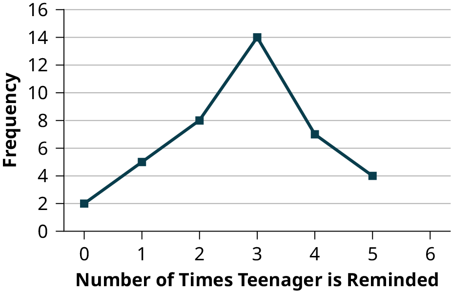
横軸に家事をするよう10代の子どもに注意する回数、縦軸に度数を取った折れ線グラフ。 — Figure 2.2図 2.2

Try Itやってみよう

In a survey, 40 people were asked how many times per year they had their car in the shop for repairs. The results are shown in Table 2.8. Construct a line graph.

ある調査で、40人に、年に何回車を修理工場に出したか尋ねた。結果を表2.8に示す。折れ線グラフを作成せよ。

Table 2.8表 2.8
Number of times in shop 修理工場に出した回数	Frequency 度数
0	7
1	10
2	14
3	9

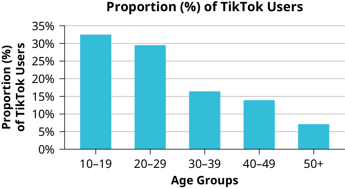
Bar graphs consist of bars that are separated from each other. The bars can be rectangles or they can be rectangular boxes (used in three-dimensional plots), and they can be vertical or horizontal. The bar graph shown in Example 2.5 has age groups represented on the x-axis and proportions on the y-axis.

英語のヒント

棒グラフは、互いに離れた棒からなる。棒は長方形、または立体的な図の場合には直方体であり、縦向きにも横向きにもできる。例題2.5の棒グラフは、x軸に年齢層、y軸に割合を示す。

Example 2.5例題 2.5

The percentage of U.S.-based TikTok users by age is shown in Table 2.9. Construct a bar graph using this data.

米国在住のTikTok利用者の年齢別の百分率を表2.9に示す。このデータで棒グラフを作成せよ。

Table 2.9表 2.9
Age groups 年齢層	Proportion (%) of TikTok users TikTok利用者の割合（％）
10–19	32.5%
20–29	29.5%
30–39	16.4%
40–49	13.9%
50+	7.1%

Solution解き方

年齢層ごとのTikTok利用者の百分率を示す棒グラフ。縦軸は0～35％を5％刻みで示す。10～19歳の棒は32％、20～29歳は29％、30～39歳は16％、40～49歳は14％、50歳以上は7％の高さである。 — Figure 2.3図 2.3

Try Itやってみよう

The population in Park City is made up of children, working-age adults, and retirees. Table 2.10 shows the three age groups, the number of people in the town from each age group, and the proportion (%) of people in each age group. Construct a bar graph showing the proportions.

パークシティの人口は、子ども、労働年齢の成人、退職者からなる。表2.10は、この3つの年齢層と、各層の町の人数および割合（％）を示す。割合を示す棒グラフを作成せよ。

Table 2.10表 2.10
Age groups 年齢層	Number of people 人数	Proportion of population 人口に占める割合
Children 子ども	67,059	19%
Working-age adults 労働年齢の成人	152,198	43%
Retirees 退職者	131,662	38%

Example 2.6例題 2.6

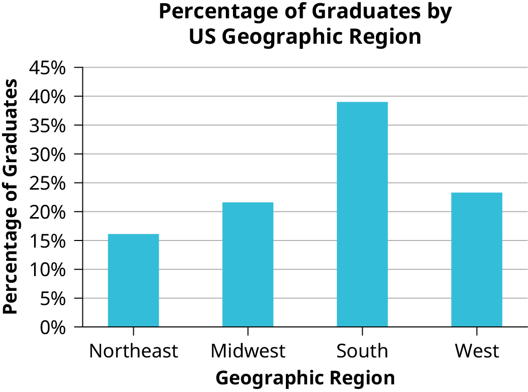
The columns in Table 2.11 show the projected data for the year 2030 for the number and percentages of high school graduates by geographic region in the United States. Create a bar graph for this data with the geographic region (qualitative data) on the x-axis and the percentage of high school data (quantitative data) on the y-axis.

表2.11の各列は、2030年の米国の高校卒業者数と百分率の予測を地域別に示す。このデータについて、x軸に地域（質的データ）、y軸に高校卒業者の百分率（量的データ）を取った棒グラフを作成せよ。

Table 2.11表 2.11
Region 地域	Number of Graduates 卒業者数	Percentage of Graduates 卒業者の百分率
Northeast 北東部	517,720	16.1%
Midwest 中西部	695,170	21.6%
South 南部	1,253,540	39.0%
West 西部	749,400	23.3%

Solution解き方

地域別の卒業者の百分率を示す棒グラフ。縦軸は0～45％を5％刻みで示す。北東部の棒は16％、中西部は22％、南部は39％、西部は23％の高さである。 — Figure 2.4図 2.4

Try Itやってみよう

Park city is broken down into six voting districts. The table shows the percent of the total registered voter population that lives in each district as well as the percent total of the entire population that lives in each district. Construct a bar graph that shows the registered voter population by district.

パークシティは6つの投票地区に分かれる。表は、登録有権者全体に対して各地区の登録有権者が占める百分率と、市の全人口に対して各地区の人口が占める百分率を示す。地区別の登録有権者人口を示す棒グラフを作成せよ。

Table 2.12表 2.12
District 地区	Registered voter population 登録有権者人口	Overall city population 市全体の人口
1	15.5%	19.4%
2	12.2%	15.6%
3	9.8%	9.0%
4	17.4%	18.5%
5	22.8%	20.7%
6	22.3%	16.8%

Losses 敗戦数	Wins 勝利数	Season シーズン	Losses 敗戦数	Wins 勝利数	Season シーズン
34	48	1	41	41	22
34	48	2	39	43	23
46	36	3	44	38	24
46	36	4	39	43	25
36	46	5	25	57	26
47	35	6	40	42	27
51	31	7	36	46	28
53	29	8	26	56	29
51	31	9	32	50	30
41	41	10	19	31	31
36	46	11	54	28	32
32	50	12	57	25	33
51	31	13	49	33	34
40	42	14	47	35	35
39	43	15	54	28	36
42	40	16	69	13	37
48	34	17	56	26	38
32	50	18	52	30	39
25	57	19	45	37	40
32	50	20	35	47	41
30	52	21	29	53	42

Losses 敗戦数	Wins 勝利数	Season シーズン	Losses 敗戦数	Wins 勝利数	Season シーズン
34	48	1	41	41	22
34	48	2	39	43	23
46	36	3	44	38	24
46	36	4	39	43	25
36	46	5	25	57	26
47	35	6	40	42	27
51	31	7	36	46	28
53	29	8	26	56	29
51	31	9	32	50	30
41	41	10	19	31	31
36	46	11	54	28	32
32	50	12	57	25	33
51	31	13	49	33	34
40	42	14	47	35	35
39	43	15	54	28	36
42	40	16	69	13	37
48	34	17	56	26	38
32	50	18	52	30	39
25	57	19	45	37	40
32	50	20	35	47	41
30	52	21	29	53	42

第2章記述統計

2.1 Stem-and-Leaf Graphs (Stemplots), Line Graphs, and Bar Graphs2.1 幹葉図、折れ線グラフ、棒グラフ

Stem-and-Leaf Graph幹葉図

Presidential Ages at Inauguration大統領の就任時の年齢

Presidential Age at Death大統領の死亡時の年齢

2.1 Stem-and-Leaf Graphs (Stemplots), Line Graphs, and Bar Graphs2.1　幹葉図、折れ線グラフ、棒グラフ

Losses 敗戦数	Wins 勝利数	Season シーズン	Losses 敗戦数	Wins 勝利数	Season シーズン
34	48	1	41	41	22
34	48	2	39	43	23
46	36	3	44	38	24
46	36	4	39	43	25
36	46	5	25	57	26
47	35	6	40	42	27
51	31	7	36	46	28
53	29	8	26	56	29
51	31	9	32	50	30
41	41	10	19	31	31
36	46	11	54	28	32
32	50	12	57	25	33
51	31	13	49	33	34
40	42	14	47	35	35
39	43	15	54	28	36
42	40	16	69	13	37
48	34	17	56	26	38
32	50	18	52	30	39
25	57	19	45	37	40
32	50	20	35	47	41
30	52	21	29	53	42