第2章記述統計
Frequency Polygons度数折れ線
Frequency polygons are analogous to line graphs, and just as line graphs make continuous data visually easy to interpret, so too do frequency polygons.
英語のヒント
度数折れ線は折れ線グラフに類似しており、折れ線グラフと同じように、連続データを視覚的に解釈しやすくする。
To construct a frequency polygon, first examine the data and decide on the number of intervals, or class intervals, to use on the x-axis and y-axis. After choosing the appropriate ranges, begin plotting the data points. After all the points are plotted, draw line segments to connect them.
度数折れ線を作るには、まずデータを調べ、x軸とy軸で使う区間、すなわち階級区間の数を決める。適切な範囲を選んだら、データの点を打つ。すべての点を打った後、線分で結ぶ。
Example 2.10例題 2.10
A frequency polygon was constructed from the frequency table below.
以下の度数表から、度数折れ線を作成した。
Frequency Distribution for Calculus Final Test Scores 微積分の期末試験の点数の度数分布 |
|||
|---|---|---|---|
Lower Bound 下限 |
Upper Bound 上限 |
Frequency 度数 |
Cumulative Frequency 累積度数 |
49.5 |
59.5 |
5 |
5 |
59.5 |
69.5 |
10 |
15 |
69.5 |
79.5 |
30 |
45 |
79.5 |
89.5 |
40 |
85 |
89.5 |
99.5 |
15 |
100 |
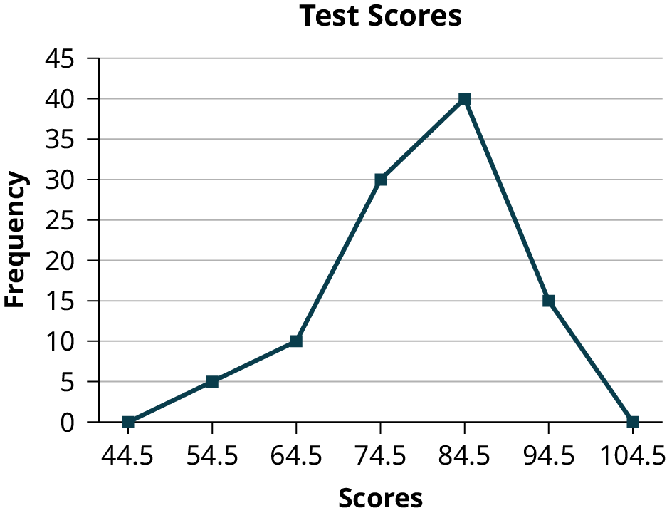
Figure 2.15図 2.15
The first label on the x-axis is 44.5. This represents an interval extending from 39.5 to 49.5. Since the lowest test score is 54.5, this interval is used only to allow the graph to touch the x-axis. The point labeled 54.5 represents the next interval, or the first “real” interval from the table, and contains five scores. This reasoning is followed for each of the remaining intervals with the point 104.5 representing the interval from 99.5 to 109.5. Again, this interval contains no data and is only used so that the graph will touch the x-axis. Looking at the graph, we say that this distribution is skewed because one side of the graph does not mirror the other side.
英語のヒント
x軸の最初の表示は44.5であり、39.5~49.5の区間を表す。試験の最低点は54.5なので、この区間はグラフをx軸に接触させるためだけに用いる。54.5と表示した点は、次の区間、つまり表の最初の「実際の」区間を表し、5つの点数が入る。残りの区間も同じ考え方で扱い、104.5の点は99.5~109.5を表す。この区間にもデータはなく、グラフをx軸に接触させるためだけに用いる。グラフを見ると、左右が鏡映対称ではないため、この分布は歪んでいるという。
Frequency polygons are useful for comparing distributions. This is achieved by overlaying the frequency polygons drawn for different data sets.
英語のヒント
度数折れ線は、分布の比較に役立つ。異なるデータセットの度数折れ線を重ね合わせることで比較できる。
Example 2.11例題 2.11
We will construct an overlay frequency polygon comparing the scores from Example 2.10 with the students’ final numeric grade.
例題2.10の点数と、学生の最終成績の数値を比較するため、度数折れ線を重ね合わせて描く。
Frequency Distribution for Calculus Final Test Scores 微積分の期末試験の点数の度数分布 |
|||
|---|---|---|---|
Lower Bound 下限 |
Upper Bound 上限 |
Frequency 度数 |
Cumulative Frequency 累積度数 |
49.5 |
59.5 |
5 |
5 |
59.5 |
69.5 |
10 |
15 |
69.5 |
79.5 |
30 |
45 |
79.5 |
89.5 |
40 |
85 |
89.5 |
99.5 |
15 |
100 |
Frequency Distribution for Calculus Final Grades 微積分の最終成績の度数分布 |
|||
|---|---|---|---|
Lower Bound 下限 |
Upper Bound 上限 |
Frequency 度数 |
Cumulative Frequency 累積度数 |
49.5 |
59.5 |
10 |
10 |
59.5 |
69.5 |
10 |
20 |
69.5 |
79.5 |
30 |
50 |
79.5 |
89.5 |
45 |
95 |
89.5 |
99.5 |
5 |
100 |
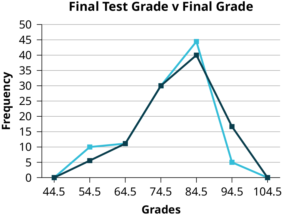
Figure 2.16図 2.16
Constructing a Time Series Graph時系列グラフの作成
Suppose that we want to study the temperature range of a region for an entire month. Every day at noon we note the temperature and write this down in a log. A variety of statistical studies could be done with this data. We could find the mean or the median temperature for the month. We could construct a histogram displaying the number of days that temperatures reach a certain range of values. However, all of these methods ignore a portion of the data that we have collected.
英語のヒント
ある地域の気温の範囲を、1か月間調べたいとする。毎日正午に気温を観測し、記録簿に書く。このデータで、さまざまな統計的な検討ができる。その月の平均気温や中央値を求めたり、特定の気温の範囲に入る日数をヒストグラムで示したりできる。しかし、これらの方法はどれも、集めたデータの一部を無視している。
One feature of the data that we may want to consider is that of time. Since each date is paired with the temperature reading for the day, we don‘t have to think of the data as being random. We can instead use the times given to impose a chronological order on the data. A graph that recognizes this ordering and displays the changing temperature as the month progresses is called a time series graph.
英語のヒント
注目したいデータの特徴の1つは、時間である。各日付はその日の気温と対になっているので、データをばらばらなものと考える必要はない。与えられた時刻を使って、時間順に並べられる。この順序を踏まえ、月の進行に伴う気温の変化を示すグラフを時系列グラフという。
To construct a time series graph, we must look at both pieces of our paired data set. We start with a standard Cartesian coordinate system. The horizontal axis is used to plot the date or time increments, and the vertical axis is used to plot the values of the variable that we are measuring. By doing this, we make each point on the graph correspond to a date and a measured quantity. The points on the graph are typically connected by straight lines in the order in which they occur.
英語のヒント
時系列グラフを作るには、対になったデータの両方を見る。通常の直交座標系を用い、横軸には日付や時間の刻み、縦軸には測定する変数の値を取る。こうすると、グラフの各点は日付と測定量の組に対応する。通常は、それらの点を出来事の順に直線で結ぶ。
Example 2.12例題 2.12
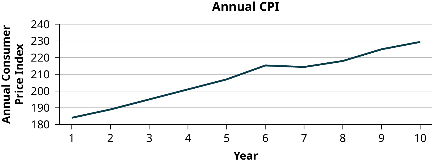
The following data shows the Annual Consumer Price Index, each month, for ten years. Construct a time series graph for the Annual Consumer Price Index data only.
以下は、10年間の各月および年平均の消費者物価指数を示すデータである。年平均の消費者物価指数のデータだけで、時系列グラフを作成せよ。
Year 年 |
Jan 1月 |
Feb 2月 |
Mar 3月 |
Apr 4月 |
May 5月 |
Jun 6月 |
Jul 7月 |
|---|---|---|---|---|---|---|---|
1 |
181.7 |
183.1 |
184.2 |
183.8 |
183.5 |
183.7 |
183.9 |
2 |
185.2 |
186.2 |
187.4 |
188.0 |
189.1 |
189.7 |
189.4 |
3 |
190.7 |
191.8 |
193.3 |
194.6 |
194.4 |
194.5 |
195.4 |
4 |
198.3 |
198.7 |
199.8 |
201.5 |
202.5 |
202.9 |
203.5 |
5 |
202.416 |
203.499 |
205.352 |
206.686 |
207.949 |
208.352 |
208.299 |
6 |
211.080 |
211.693 |
213.528 |
214.823 |
216.632 |
218.815 |
219.964 |
7 |
211.143 |
212.193 |
212.709 |
213.240 |
213.856 |
215.693 |
215.351 |
8 |
216.687 |
216.741 |
217.631 |
218.009 |
218.178 |
217.965 |
218.011 |
9 |
220.223 |
221.309 |
223.467 |
224.906 |
225.964 |
225.722 |
225.922 |
10 |
226.665 |
227.663 |
229.392 |
230.085 |
229.815 |
229.478 |
229.104 |
Year 年 |
Aug 8月 |
Sep 9月 |
Oct 10月 |
Nov 11月 |
Dec 12月 |
Annual 年平均 |
|---|---|---|---|---|---|---|
1 |
184.6 |
185.2 |
185.0 |
184.5 |
184.3 |
184.0 |
2 |
189.5 |
189.9 |
190.9 |
191.0 |
190.3 |
188.9 |
3 |
196.4 |
198.8 |
199.2 |
197.6 |
196.8 |
195.3 |
4 |
203.9 |
202.9 |
201.8 |
201.5 |
201.8 |
201.6 |
5 |
207.917 |
208.490 |
208.936 |
210.177 |
210.036 |
207.342 |
6 |
219.086 |
218.783 |
216.573 |
212.425 |
210.228 |
215.303 |
7 |
215.834 |
215.969 |
216.177 |
216.330 |
215.949 |
214.537 |
8 |
218.312 |
218.439 |
218.711 |
218.803 |
219.179 |
218.056 |
9 |
226.545 |
226.889 |
226.421 |
226.230 |
225.672 |
224.939 |
10 |
230.379 |
231.407 |
231.317 |
230.221 |
229.601 |
229.594 |