第2章記述統計
Explanation of the standard deviation calculation shown in the table表に示した標準偏差の計算の説明
The deviations show how spread out the data are about the mean. The data value 11.5 is farther from the mean than is the data value 11 which is indicated by the deviations 0.97 and 0.47. A positive deviation occurs when the data value is greater than the mean, whereas a negative deviation occurs when the data value is less than the mean. The deviation is –1.525 for the data value nine. If you add the deviations, the sum is always zero. (For Example 2.32, there are n = 20 deviations.) So you cannot simply add the deviations to get the spread of the data. By squaring the deviations, you make them positive numbers, and the sum will also be positive. The variance, then, is the average squared deviation.
偏差は、データが平均の周りにどれほど散らばっているかを示す。値11.5は値11よりも平均から遠く、そのことが偏差0.97と0.47に表れている。データの値が平均より大きければ偏差は正、小さければ負になる。値9の偏差は−1.525である。偏差を合計すると、必ず0になる。(例2.32では、偏差はn=20個ある。)したがって、偏差を単純に足すだけでは散らばりを求められない。偏差を2乗すれば正の数になり、合計も正になる。こうして得る分散は、偏差の2乗の平均である。
The variance is a squared measure and does not have the same units as the data. Taking the square root solves the problem. The standard deviation measures the spread in the same units as the data.
分散は2乗された尺度なので、元のデータと単位が異なる。平方根を取ると、この問題が解消する。標準偏差は、データと同じ単位で散らばりを測る。
Notice that instead of dividing by n = 20, the calculation divided by n – 1 = 20 – 1 = 19 because the data is a sample. For the sample variance, we divide by the sample size minus one (n – 1). Why not divide by n? The answer has to do with the population variance. The sample variance is an estimate of the population variance. Based on the theoretical mathematics that lies behind these calculations, dividing by (n – 1) gives a better estimate of the population variance.
英語のヒント
この計算ではn=20ではなく、n−1=20−1=19で割った点に注意しよう。データが標本だからである。標本分散では、標本の大きさから1を引いたn−1で割る。なぜnで割らないのか。その答えは母分散に関係する。標本分散は母分散の推定値である。計算の背後にある数学理論によれば、n−1で割る方が母分散のよりよい推定値を得られる。
The standard deviation, s or σ, is either zero or larger than zero. Describing the data with reference to the spread is called "variability". The variability in data depends upon the method by which the outcomes are obtained; for example, by measuring or by random sampling. When the standard deviation is zero, there is no spread; that is, the all the data values are equal to each other. The standard deviation is small when the data are all concentrated close to the mean, and is larger when the data values show more variation from the mean. When the standard deviation is a lot larger than zero, the data values are very spread out about the mean; outliers can make s or σ very large.
標準偏差sまたはσは、0以上である。データの散らばりに着目した性質を「ばらつき」という。ばらつきは、測定や無作為抽出など、結果を得る方法に左右される。標準偏差が0なら散らばりはなく、すべての値が互いに等しい。すべての値が平均の近くに集中していれば標準偏差は小さく、平均からの変動が大きいほど標準偏差も大きい。標準偏差が0を大きく上回るとき、データは平均の周りに広く散らばっている。外れ値によってsやσが非常に大きくなることもある。
The standard deviation, when first presented, can seem unclear. By graphing your data, you can get a better "feel" for the deviations and the standard deviation. You will find that in symmetrical distributions, the standard deviation can be very helpful but in skewed distributions, the standard deviation may not be much help. The reason is that the two sides of a skewed distribution have different spreads. In a skewed distribution, it is better to look at the first quartile, the median, the third quartile, the smallest value, and the largest value. Because numbers can be confusing, always graph your data. Display your data in a histogram or a box plot.
英語のヒント
初めて標準偏差に触れると、分かりにくく感じるかもしれない。データをグラフにすれば、偏差や標準偏差をより実感しやすくなる。対称な分布では標準偏差はとても役立つが、歪んだ分布ではあまり役立たないことがある。分布の左右で散らばりが異なるからである。歪んだ分布では、第1四分位数、中央値、第3四分位数、最小値、最大値を見る方がよい。数値だけでは分かりにくいので、必ずデータをグラフにしよう。ヒストグラムや箱ひげ図で示すとよい。
Example 2.33例題 2.33
Use the following data (first exam scores) from Professor Dean's spring pre-calculus class:
ディーン教授の春学期の微積分準備クラスで得た、次のデータ(第1回試験の得点)を使う。
33; 42; 49; 49; 53; 55; 55; 61; 63; 67; 68; 68; 69; 69; 72; 73; 74; 78; 80; 83; 88; 88; 88; 90; 92; 94; 94; 94; 94; 96; 100
- Create a chart containing the data, frequencies, relative frequencies, and cumulative relative frequencies to three decimal places.データ、度数、相対度数、累積相対度数を小数第3位まで示した表を作成せよ。
- Calculate the following to one decimal place using a TI-83+ or TI-84 calculator:TI-83+またはTI-84で、次の値を小数第1位まで求めよ。
- The sample mean標本平均
- The sample standard deviation標本標準偏差
- The median中央値
- The first quartile第1四分位数
- The third quartile第3四分位数
- IQR四分位範囲(IQR)
- Construct a box plot and a histogram on the same set of axes. Make comments about the box plot, the histogram, and the chart.同じ座標軸上に箱ひげ図とヒストグラムを描け。箱ひげ図、ヒストグラム、表について気づいた点を述べよ。
Solution解き方
- See Table 2.70表2.70を参照。
- The sample mean = 73.5標本平均=73.5
- The sample standard deviation = 17.9標本標準偏差=17.9
- The median = 73中央値=73
- The first quartile = 61第1四分位数=61
- The third quartile = 90第3四分位数=90
- IQR = 90 – 61 = 29IQR=90−61=29
- The x-axis goes from 32.5 to 100.5; y-axis goes from –2.4 to 15 for the histogram. The number of intervals is five, so the width of an interval is (100.5 – 32.5) divided by five, is equal to 13.6. Endpoints of the intervals are as follows: the starting point is 32.5, 32.5 + 13.6 = 46.1, 46.1 + 13.6 = 59.7, 59.7 + 13.6 = 73.3, 73.3 + 13.6 = 86.9, 86.9 + 13.6 = 100.5 = the ending value; No data values fall on an interval boundary.ヒストグラムのx軸は32.5~100.5、y軸は−2.4~15とする。階級数は5なので、階級幅は(100.5−32.5)÷5=13.6である。階級の端は、始点32.5、32.5+13.6=46.1、46.1+13.6=59.7、59.7+13.6=73.3、73.3+13.6=86.9、86.9+13.6=100.5(終点)となる。階級の境界に一致するデータの値はない。
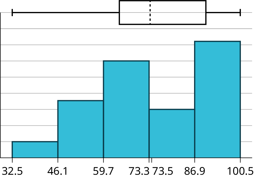

Figure 2.57図 2.57
Data データ |
Frequency 度数 |
Relative Frequency 相対度数 |
Cumulative Relative Frequency 累積相対度数 |
|---|---|---|---|
33 |
1 |
0.032 |
0.032 |
42 |
1 |
0.032 |
0.064 |
49 |
2 |
0.065 |
0.129 |
53 |
1 |
0.032 |
0.161 |
55 |
2 |
0.065 |
0.226 |
61 |
1 |
0.032 |
0.258 |
63 |
1 |
0.032 |
0.29 |
67 |
1 |
0.032 |
0.322 |
68 |
2 |
0.065 |
0.387 |
69 |
2 |
0.065 |
0.452 |
72 |
1 |
0.032 |
0.484 |
73 |
1 |
0.032 |
0.516 |
74 |
1 |
0.032 |
0.548 |
78 |
1 |
0.032 |
0.580 |
80 |
1 |
0.032 |
0.612 |
83 |
1 |
0.032 |
0.644 |
88 |
3 |
0.097 |
0.741 |
90 |
1 |
0.032 |
0.773 |
92 |
1 |
0.032 |
0.805 |
94 |
4 |
0.129 |
0.934 |
96 |
1 |
0.032 |
0.966 |
100 |
1 |
0.032 |
0.998 (Why isn't this value 1?) 0.998(なぜ1にならないのか。) |
The long left whisker in the box plot is reflected in the left side of the histogram. The spread of the exam scores in the lower 50% is greater (73 – 33 = 40) than the spread in the upper 50% (100 – 73 = 27). The histogram, box plot, and chart all reflect this. There are a substantial number of A and B grades (80s, 90s, and 100). The histogram clearly shows this. The box plot shows us that the middle 50% of the exam scores (IQR = 29) are Ds, Cs, and Bs. The box plot also shows us that the lower 25% of the exam scores are Ds and Fs.
英語のヒント
箱ひげ図の長い左ひげに対応して、ヒストグラムも左側へ広がっている。得点の下位50%の範囲は73−33=40で、上位50%の範囲100−73=27より広い。このことはヒストグラム、箱ひげ図、表のすべてに表れている。AとBの成績(80点台、90点台、100点)がかなり多いことも、ヒストグラムから明瞭に分かる。箱ひげ図は、中央50%の得点(IQR=29)がD、C、Bに属し、下位25%の得点がDとFに属することを示している。