第2章記述統計

References参考文献

Data on annual homicides in Detroit, 1961–73, from Gunst & Mason’s book ‘Regression Analysis and its Application’, Marcel Dekker

1961～1973年のデトロイトの年間殺人件数。GunstとMasonの著書『回帰分析とその応用』（Marcel Dekker）による。

“Timeline: Guide to the U.S. Presidents: Information on every president’s birthplace, political party, term of office, and more.” Scholastic, 2013. Available online at http://www.scholastic.com/teachers/article/timeline-guide-us-presidents (accessed April 3, 2013).

「年表：米国大統領ガイド―各大統領の出生地、政党、在任期間など」、Scholastic、2013年。http://www.scholastic.com/teachers/article/timeline-guide-us-presidents（2013年4月3日閲覧）。

“Presidents.” Fact Monster. Pearson Education, 2007. Available online at http://www.factmonster.com/ipka/A0194030.html (accessed April 3, 2013).

「大統領」、Fact Monster、Pearson Education、2007年。http://www.factmonster.com/ipka/A0194030.html（2013年4月3日閲覧）。

“Food Security Statistics.” Food and Agriculture Organization of the United Nations. Available online at http://www.fao.org/economic/ess/ess-fs/en/ (accessed April 3, 2013).

「食料安全保障統計」、国際連合食糧農業機関。http://www.fao.org/economic/ess/ess-fs/en/（2013年4月3日閲覧）。

“Consumer Price Index.” United States Department of Labor: Bureau of Labor Statistics. Available online at http://data.bls.gov/pdq/SurveyOutputServlet (accessed April 3, 2013).

「消費者物価指数」、米国労働省労働統計局。http://data.bls.gov/pdq/SurveyOutputServlet（2013年4月3日閲覧）。

“CO2 emissions (kt).” The World Bank, 2013. Available online at http://databank.worldbank.org/data/home.aspx (accessed April 3, 2013).

「CO2排出量（千トン）」、世界銀行、2013年。http://databank.worldbank.org/data/home.aspx（2013年4月3日閲覧）。

“Births Time Series Data.” General Register Office For Scotland, 2013. Available online at http://www.gro-scotland.gov.uk/statistics/theme/vital-events/births/time-series.html (accessed April 3, 2013).

「出生の時系列データ」、スコットランド登録局、2013年。http://www.gro-scotland.gov.uk/statistics/theme/vital-events/births/time-series.html（2013年4月3日閲覧）。

“Demographics: Children under the age of 5 years underweight.” Indexmundi. Available online at http://www.indexmundi.com/g/r.aspx?t=50&v=2224&aml=en (accessed April 3, 2013).

「人口統計：低体重の5歳未満の子ども」、Indexmundi。http://www.indexmundi.com/g/r.aspx?t=50&v=2224&aml=en（2013年4月3日閲覧）。

Gunst, Richard, Robert Mason. Regression Analysis and Its Application: A Data-Oriented Approach. CRC Press: 1980.

Richard Gunst、Robert Mason『回帰分析とその応用：データを重視した方法』、CRC Press、1980年。

“Overweight and Obesity: Adult Obesity Facts.” Centers for Disease Control and Prevention. Available online at http://www.cdc.gov/obesity/data/adult.html (accessed September 13, 2013).

「過体重と肥満：成人の肥満に関する情報」、疾病対策予防センター。http://www.cdc.gov/obesity/data/adult.html（2013年9月13日閲覧）。

Chapter Review章の復習

A histogram is a graphic version of a frequency distribution. The graph consists of bars of equal width drawn adjacent to each other. The horizontal scale represents classes of quantitative data values and the vertical scale represents frequencies. The heights of the bars correspond to frequency values. Histograms are typically used for large, continuous, quantitative data sets. A frequency polygon can also be used when graphing large data sets with data points that repeat. The data usually goes on y-axis with the frequency being graphed on the x-axis. Time series graphs can be helpful when looking at large amounts of data for one variable over a period of time.

ヒストグラムは、度数分布を図にしたものである。同じ幅の棒を互いに接して描き、横の尺度は量的データの値の階級、縦の尺度は度数を表す。棒の高さは度数に対応する。一般に、大規模で連続的な量的データに用いる。同じ値が繰り返される大きなデータセットを図示する場合には、度数折れ線も使える。通常、データをy軸、度数をx軸に取る。1つの変数について、ある期間の大量のデータを見るときには、時系列グラフが役立つ。

Exercises 14–24練習問題 14–24

Exercise 14問題 14

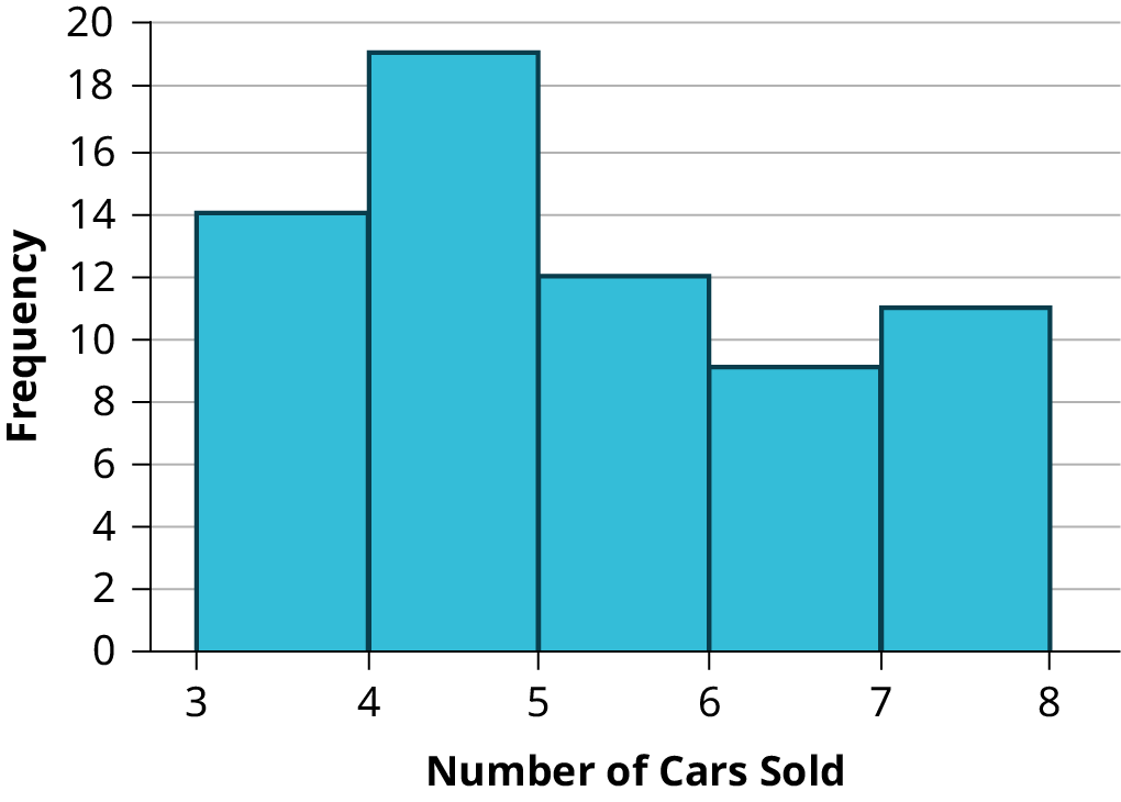
Sixty-five randomly selected car salespersons were asked the number of cars they generally sell in one week. Fourteen people answered that they generally sell three cars; nineteen generally sell four cars; twelve generally sell five cars; nine generally sell six cars; eleven generally sell seven cars. Complete the table.

無作為に選んだ自動車販売員65人に、通常1週間で何台売るか尋ねた。14人は3台、19人は4台、12人は5台、9人は6台、11人は7台と答えた。表を完成させよ。

Table 2.30表 2.30
Data Value (# cars) データの値（車の台数）	Frequency 度数	Relative Frequency 相対度数	Cumulative Relative Frequency 累積相対度数

Exercise 15問題 15

What does the frequency column in Table 2.30 sum to? Why?

表2.30の度数の列の合計はいくつか。理由も述べよ。

Solution解き方

Exercise 16問題 16

What does the relative frequency column in Table 2.30 sum to? Why?

表2.30の相対度数の列の合計はいくつか。理由も述べよ。

Exercise 17問題 17

What is the difference between relative frequency and frequency for each data value in Table 2.30?

表2.30の各データの値について、相対度数と度数はどう違うか。

Solution解き方

The relative frequency shows the proportion of data points that have each value. The frequency tells the number of data points that have each value.

相対度数は、それぞれの値を持つデータの割合を示す。度数は、それぞれの値を持つデータの個数を示す。

Exercise 18問題 18

What is the difference between cumulative relative frequency and relative frequency for each data value?

各データの値について、累積相対度数と相対度数はどう違うか。

Exercise 19問題 19

To construct the histogram for the data in Table 2.30, determine appropriate minimum and maximum x and y values and the scaling. Sketch the histogram. Label the horizontal and vertical axes with words. Include numerical scaling.

表2.30のデータのヒストグラムを作るため、xとyの適切な最小値・最大値と目盛りを決めよ。ヒストグラムを描き、横軸と縦軸に何を表すかを言葉で記し、数値の目盛りも入れよ。

Solution解き方

Answers will vary. One possible histogram is shown:

答えはさまざまである。ヒストグラムの一例を示す。

自動車の販売データに対応するヒストグラム。横軸は販売台数を3～8の範囲で1刻み、縦軸は度数を0～20の範囲で2刻みに示す。3～4の棒の高さは14、4～5は19、5～6は12、6～7は9、7～8は11である。 — Figure 2.19図 2.19

Exercise 20問題 20

Construct a frequency polygon for the following:

以下について、度数折れ線を作成せよ。

Pulse Rates for Females
女性の脈拍数

Frequency
度数

60–69

12

70–79

14

80–89

11

90–99

1

100–109

1

110–119

0

120–129

1

Table 2.31表 2.31
Actual Speed in a 30 MPH Zone
制限速度が時速30マイルの区域での実際の速度

Frequency
度数

42–45

25

46–49

14

50–53

7

54–57

3

58–61

1

Table 2.32表 2.32
Tar (mg) in Nonfiltered Cigarettes
フィルターなしのたばこに含まれるタール（mg）

Frequency
度数

10–13

1

14–17

0

18–21

15

22–25

7

26–29

2

Table 2.33表 2.33

Table 2.31表 2.31
Pulse Rates for Females 女性の脈拍数	Frequency 度数
60–69	12
70–79	14
80–89	11
90–99	1
100–109	1
110–119	0
120–129	1

Table 2.32表 2.32
Actual Speed in a 30 MPH Zone 制限速度が時速30マイルの区域での実際の速度	Frequency 度数
42–45	25
46–49	14
50–53	7
54–57	3
58–61	1

Table 2.33表 2.33
Tar (mg) in Nonfiltered Cigarettes フィルターなしのたばこに含まれるタール（mg）	Frequency 度数
10–13	1
14–17	0
18–21	15
22–25	7
26–29	2

Exercise 21問題 21

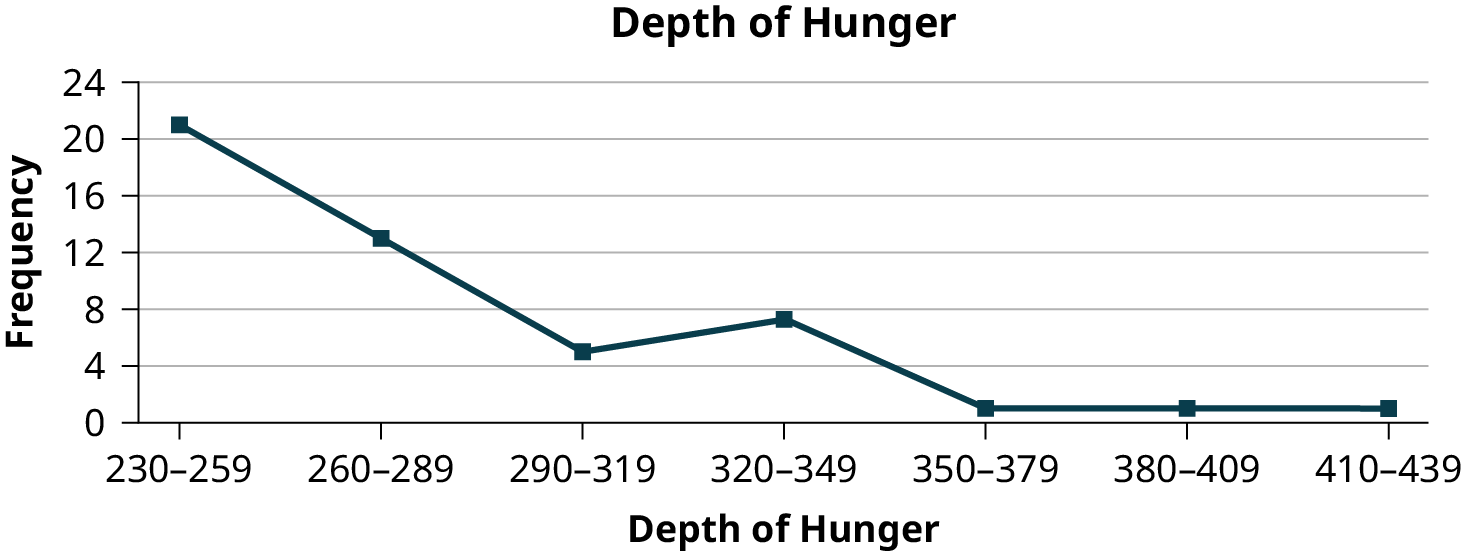
Construct a frequency polygon from the frequency distribution for the 50 highest ranked countries for depth of hunger.

飢餓の深刻さで上位に位置する50か国の度数分布から、度数折れ線を作成せよ。

Table 2.34表 2.34
Depth of Hunger 飢餓の深刻さ	Frequency 度数
230–259	21
260–289	13
290–319	5
320–349	7
350–379	1
380–409	1
410–439	1

Solution解き方

Find the midpoint for each class. These will be graphed on the x-axis. The frequency values will be graphed on the y-axis values.

各階級の中点を求め、x軸に取る。度数の値はy軸に取る。

与えられたデータに対応する度数折れ線。横軸は飢餓の深刻さ、縦軸は度数である。 — Figure 2.20図 2.20

Exercise 22問題 22

Use the two frequency tables to compare the life expectancy of males and females from 20 randomly selected countries. Include an overlayed frequency polygon and discuss the shapes of the distributions, the center, the spread, and any outliers. What can we conclude about the life expectancy of females compared to males?

英語のヒント

2つの度数表を使い、無作為に選んだ20か国の男性と女性の平均余命を比較せよ。度数折れ線を重ねて描き、分布の形、中心、散らばり、外れ値について論じよ。女性の平均余命を男性と比較して、何が結論できるか。

Table 2.35表 2.35
Life Expectancy at Birth – Females 出生時平均余命―女性	Frequency 度数
49–55	3
56–62	3
63–69	1
70–76	3
77–83	8
84–90	2

Table 2.36表 2.36
Life Expectancy at Birth – Males 出生時平均余命―男性	Frequency 度数
49–55	3
56–62	3
63–69	1
70–76	1
77–83	7
84–90	5

Exercise 23問題 23

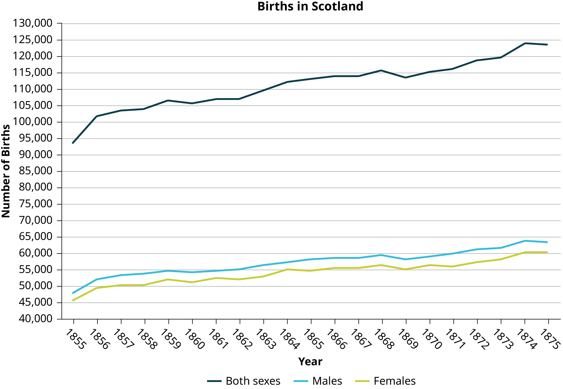
Construct a times series graph for (a) the number of male births, (b) the number of female births, and (c) the total number of births.

（a）男児出生数、（b）女児出生数、（c）出生総数について、時系列グラフを作成せよ。

Table 2.37表 2.37
Sex/Year 性別／年	1855	1856	1857	1858	1859	1860	1861
Female 女性	45,545	49,582	50,257	50,324	51,915	51,220	52,403
Male 男性	47,804	52,239	53,158	53,694	54,628	54,409	54,606
Total 合計	93,349	101,821	103,415	104,018	106,543	105,629	107,009

Table 2.38表 2.38
Sex/Year 性別／年	1862	1863	1864	1865	1866	1867	1868	1869
Female 女性	51,812	53,115	54,959	54,850	55,307	55,527	56,292	55,033
Male 男性	55,257	56,226	57,374	58,220	58,360	58,517	59,222	58,321
Total 合計	107,069	109,341	112,333	113,070	113,667	114,044	115,514	113,354

Table 2.39表 2.39
Sex/Year 性別／年	1870	1871	1872	1873	1874	1875
Female 女性	56,431	56,099	57,472	58,233	60,109	60,146
Male 男性	58,959	60,029	61,293	61,467	63,602	63,432
Total 合計	115,390	116,128	118,765	119,700	123,711	123,578

Solution解き方

表2.49、2.50、2.51のデータから作成した、スコットランドの出生数を示す折れ線グラフ。横軸は1855～1875年を1年刻み、縦軸は40,000～130,000人を5,000人刻みで示す。女児出生数の折れ線は、1855年の45,545人から1875年の60,146人へ増加する。男児出生数の折れ線は47,804人から63,432人へ、出生総数の折れ線は93,349人から123,578人へ増加する。 — Figure 2.21図 2.21

Exercise 24問題 24

The following data sets list full time police per 100,000 citizens along with homicides per 100,000 citizens for a city during the period from 1961 to 1973.

英語のヒント

以下のデータセットは、ある市の1961～1973年について、市民10万人当たりの常勤警察官数と殺人件数を示す。

Table 2.40表 2.40
Year 年	1961	1962	1963	1964	1965	1966	1967
Police 警察官	260.35	269.8	272.04	272.96	272.51	261.34	268.89
Homicides 殺人件数	8.6	8.9	8.52	8.89	13.07	14.57	21.36

Table 2.41表 2.41
Year 年	1968	1969	1970	1971	1972	1973
Police 警察官	295.99	319.87	341.43	356.59	376.69	390.19
Homicides 殺人件数	28.03	31.49	37.39	46.26	47.24	52.33

Construct a double time series graph using a common x-axis for both sets of data.
2組のデータについて、共通のx軸を使った2系列の時系列グラフを作成せよ。
Which variable increased the fastest? Explain.
どちらの変数がより速く増加したか。説明せよ。
Did the city's increase in police officers have an impact on the murder rate? Explain.
この市の警察官の増加は、殺人率に影響したか。説明せよ。