第2章記述統計
Homework宿題
Exercises 25–27練習問題 25–27
Exercise 25問題 25
Suppose that three book publishers were interested in the number of fiction paperbacks adult consumers purchase per month. Each publisher conducted a survey. In the survey, adult consumers were asked the number of fiction paperbacks they had purchased the previous month. The results are as follows:
英語のヒント
3社の出版社が、成人消費者が毎月購入するペーパーバックの小説の冊数に関心を持ったとする。各社が調査を行い、成人消費者に前月の購入冊数を尋ねた。結果は以下のとおりである。
# of books 本の冊数 |
Freq. 度数 |
Rel. Freq. 相対度数 |
|---|---|---|
0 |
10 |
|
1 |
12 |
|
2 |
16 |
|
3 |
12 |
|
4 |
8 |
|
5 |
6 |
|
6 |
2 |
|
8 |
2 |
# of books 本の冊数 |
Freq. 度数 |
Rel. Freq. 相対度数 |
|---|---|---|
0 |
18 |
|
1 |
24 |
|
2 |
24 |
|
3 |
22 |
|
4 |
15 |
|
5 |
10 |
|
7 |
5 |
|
9 |
1 |
# of books 本の冊数 |
Freq. 度数 |
Rel. Freq. 相対度数 |
|---|---|---|
0–1 |
20 |
|
2–3 |
35 |
|
4–5 |
12 |
|
6–7 |
2 |
|
8–9 |
1 |
- Find the relative frequencies for each survey. Write them in the charts.各調査の相対度数を求め、表に書き入れよ。
- Using either a graphing calculator, computer, or by hand, use the frequency column to construct a histogram for each publisher's survey. For Publishers A and B, make bar widths of one. For Publisher C, make bar widths of two.グラフ電卓、コンピューター、または手描きで、度数の列を使って各出版社の調査のヒストグラムを作成せよ。出版社AとBでは棒の幅を1、Cでは2にする。
- In complete sentences, give two reasons why the graphs for Publishers A and B are not identical.出版社AとBのグラフが同一ではない理由を2つ、完全な文で述べよ。
- Would you have expected the graph for Publisher C to look like the other two graphs? Why or why not?出版社Cのグラフは、ほかの2つに似ると予想したか。理由を説明せよ。
- Make new histograms for Publisher A and Publisher B. This time, make bar widths of two.出版社AとBのヒストグラムを作り直せ。今度は棒の幅を2にする。
- Now, compare the graph for Publisher C to the new graphs for Publishers A and B. Are the graphs more similar or more different? Explain your answer.出版社Cのグラフを、作り直したAとBのグラフと比較せよ。以前より似ているか、それとも違っているか。説明せよ。
Exercise 26問題 26
Often, cruise ships conduct all on-board transactions, with the exception of gambling, on a cashless basis. At the end of the cruise, guests pay one bill that covers all onboard transactions. Suppose that 60 single travelers and 70 couples were surveyed as to their on-board bills for a seven-day cruise from Los Angeles to the Mexican Riviera. Following is a summary of the bills for each group.
英語のヒント
クルーズ船では多くの場合、賭博を除く船内の支払いをすべてキャッシュレスで行い、航海の最後に、船内での利用すべてをまとめた請求額を支払う。ロサンゼルスからメキシカン・リビエラへ向かう7日間のクルーズについて、1人客60人とカップル70組の船内請求額を調査したとする。各集団の請求額の要約を以下に示す。
Amount($) 金額(ドル) |
Frequency 度数 |
Rel. Frequency 相対度数 |
|---|---|---|
51–100 |
5 |
|
101–150 |
10 |
|
151–200 |
15 |
|
201–250 |
15 |
|
251–300 |
10 |
|
301–350 |
5 |
Amount($) 金額(ドル) |
Frequency 度数 |
Rel. Frequency 相対度数 |
|---|---|---|
100–150 |
5 |
|
201–250 |
5 |
|
251–300 |
5 |
|
301–350 |
5 |
|
351–400 |
10 |
|
401–450 |
10 |
|
451–500 |
10 |
|
501–550 |
10 |
|
551–600 |
5 |
|
601–650 |
5 |
- Fill in the relative frequency for each group.各集団の相対度数を書き入れよ。
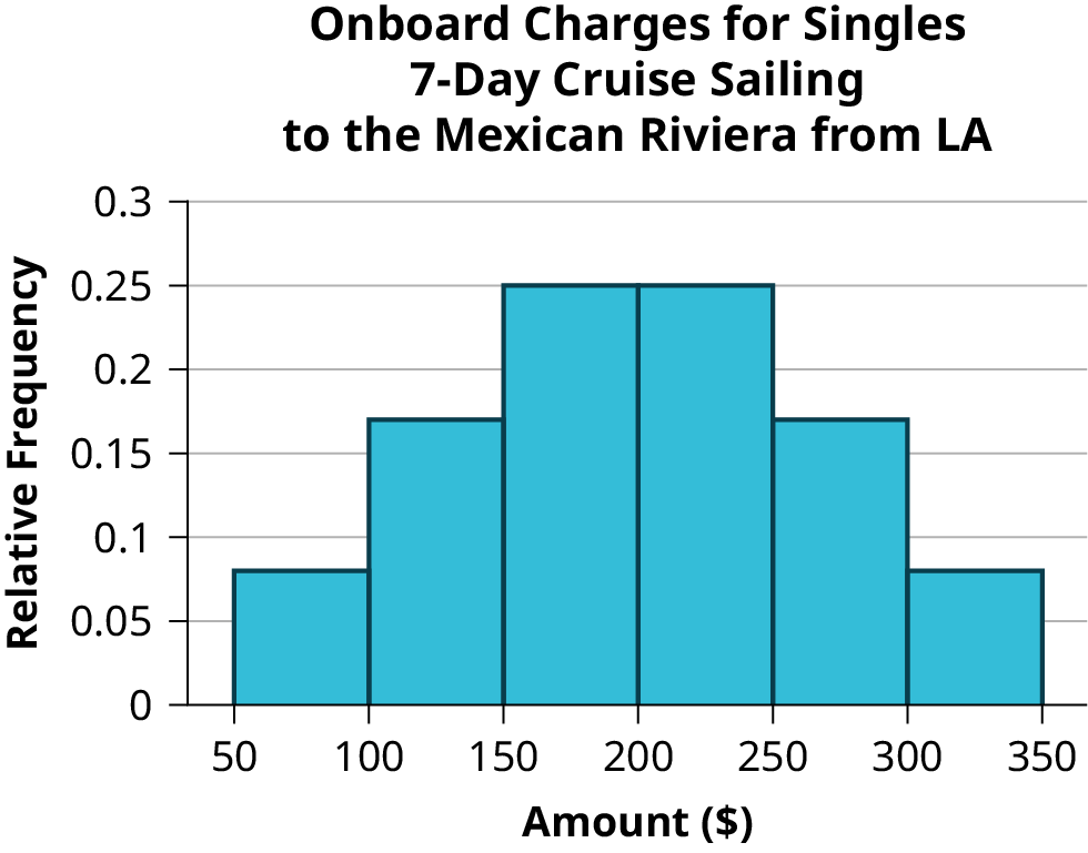
- Construct a histogram for the singles group. Scale the x-axis by $50 widths. Use relative frequency on the y-axis.1人客のヒストグラムを作成せよ。x軸は50ドル幅、y軸は相対度数とする。
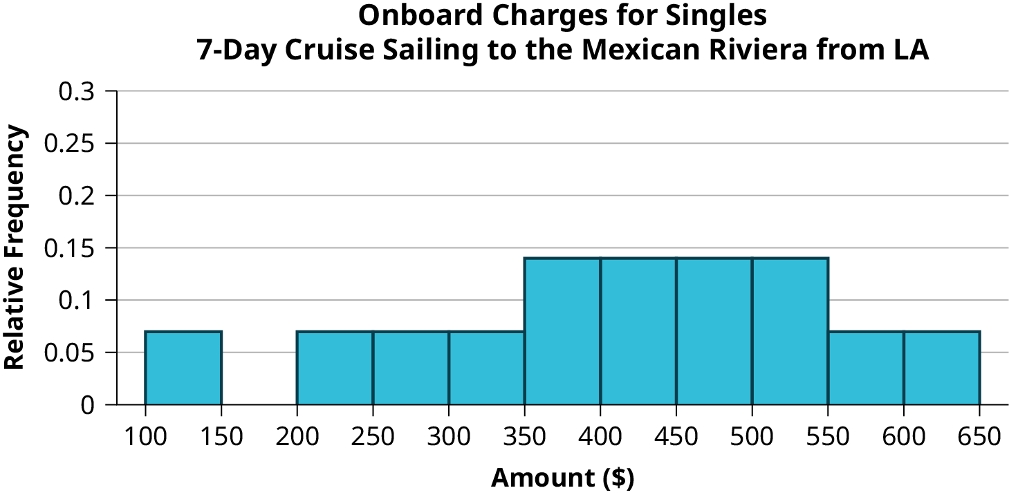
- Construct a histogram for the couples group. Scale the x-axis by $50 widths. Use relative frequency on the y-axis.カップルのヒストグラムを作成せよ。x軸は50ドル幅、y軸は相対度数とする。
- Compare the two graphs:2つのグラフを比較せよ。
- List two similarities between the graphs.グラフの共通点を2つ挙げよ。
- List two differences between the graphs.グラフの相違点を2つ挙げよ。
- Overall, are the graphs more similar or different?全体として、グラフは似ているか、異なっているか。
- Construct a new graph for the couples by hand. Since each couple is paying for two individuals, instead of scaling the x-axis by $50, scale it by $100. Use relative frequency on the y-axis.カップルのグラフを手描きで作り直せ。各カップルは2人分を支払うので、x軸は50ドル幅ではなく100ドル幅にする。y軸は相対度数とする。
- Compare the graph for the singles with the new graph for the couples:1人客のグラフと、カップルの新しいグラフを比較せよ。
- List two similarities between the graphs.グラフの共通点を2つ挙げよ。
- Overall, are the graphs more similar or different?全体として、グラフは似ているか、異なっているか。
- How did scaling the couples graph differently change the way you compared it to the singles graph?カップルのグラフの尺度を変えたことで、1人客のグラフとの比較はどう変わったか。
- Based on the graphs, do you think that individuals spend the same amount, more or less, as singles as they do person by person as a couple? Explain why in one or two complete sentences.グラフから考えて、1人客の支出は、カップルの1人当たりの支出とほぼ同じ、多い、少ないのどれだと思うか。理由を1~2文で説明せよ。
Solution解き方
Amount($) 金額(ドル) |
Frequency 度数 |
Relative Frequency 相対度数 |
|---|---|---|
51–100 |
5 |
0.08 |
101–150 |
10 |
0.17 |
151–200 |
15 |
0.25 |
201–250 |
15 |
0.25 |
251–300 |
10 |
0.17 |
301–350 |
5 |
0.08 |
Amount($) 金額(ドル) |
Frequency 度数 |
Relative Frequency 相対度数 |
|---|---|---|
100–150 |
5 |
0.07 |
201–250 |
5 |
0.07 |
251–300 |
5 |
0.07 |
301–350 |
5 |
0.07 |
351–400 |
10 |
0.14 |
401–450 |
10 |
0.14 |
451–500 |
10 |
0.14 |
501–550 |
10 |
0.14 |
551–600 |
5 |
0.07 |
601–650 |
5 |
0.07 |
- See Table 2.47 and Table 2.48.
- In the following histogram data values that fall on the right boundary are counted in the class interval, while values that fall on the left boundary are not counted (with the exception of the first interval where both boundary values are included).以下のヒストグラムでは、右側の境界上の値をその階級区間に含め、左側の境界上の値は含めない。ただし、最初の区間だけは両方の境界値を含める。Figure 2.22図 2.22
- In the following histogram, the data values that fall on the right boundary are counted in the class interval, while values that fall on the left boundary are not counted (with the exception of the first interval where values on both boundaries are included).以下のヒストグラムでは、右側の境界上の値をその階級区間に含め、左側の境界上の値は含めない。ただし、最初の区間だけは両方の境界値を含める。Figure 2.23図 2.23
- Compare the two graphs:2つのグラフを比較せよ。
- Answers may vary. Possible answers include:答えはさまざまである。解答例を以下に示す。
- Both graphs have a single peak.どちらのグラフも山は1つである。
- Both graphs use class intervals with width equal to $50.どちらも階級区間の幅は50ドルである。
- Answers may vary. Possible answers include:答えはさまざまである。解答例を以下に示す。
- The couples graph has a class interval with no values.カップルのグラフには、値のない階級区間がある。
- It takes almost twice as many class intervals to display the data for couples.カップルのデータを示すには、ほぼ2倍の階級区間が必要になる。
- Answers may vary. Possible answers include: The graphs are more similar than different because the overall patterns for the graphs are the same.答えはさまざまである。解答例:グラフ全体のパターンが同じなので、相違点より共通点の方が多い。
- Answers may vary.解答はさまざまである。
- Compare the graph for the Singles with the new graph for the Couples:1人客のグラフと、カップルの新しいグラフを比較する。
- Both graphs have a single peak.どちらのグラフも山は1つである。
- Both graphs display 6 class intervals.どちらのグラフも階級区間は6つである。
- Both graphs show the same general pattern.どちらも全体的なパターンは同じである。
- Answers may vary. Possible answers include: Although the width of the class intervals for couples is double that of the class intervals for singles, the graphs are more similar than they are different.答えはさまざまである。解答例:カップルの階級区間の幅は1人客の2倍だが、グラフは違いよりも似た点が多い。
- Answers may vary. Possible answers include: You are able to compare the graphs interval by interval. It is easier to compare the overall patterns with the new scale on the Couples graph. Because a couple represents two individuals, the new scale leads to a more accurate comparison.答えはさまざまである。解答例:区間ごとにグラフを比較できる。カップルの新しい尺度では、全体的なパターンを比較しやすい。カップルは2人を表すので、新しい尺度の方が正確な比較につながる。
- Answers may vary. Possible answers include: Based on the histograms, it seems that spending does not vary much from singles to individuals who are part of a couple. The overall patterns are the same. The range of spending for couples is approximately double the range for individuals.答えはさまざまである。解答例:ヒストグラムを見ると、1人客と、カップルの1人当たりの支出に大きな違いはなさそうである。全体的なパターンは同じで、カップルの支出の範囲は1人客の約2倍である。
Exercise 27問題 27
Twenty-five randomly selected students were asked the number of movies they watched the previous week. The results are as follows.
無作為に選んだ学生25人に、前の週に見た映画の本数を尋ねた。結果は次のとおりである。
# of movies 映画の本数 |
Frequency 度数 |
Relative Frequency 相対度数 |
Cumulative Relative Frequency 累積相対度数 |
|---|---|---|---|
0 |
5 |
||
1 |
9 |
||
2 |
6 |
||
3 |
4 |
||
4 |
1 |
- Construct a histogram of the data.データのヒストグラムを作成せよ。
- Complete the columns of the chart.表の各列を完成させよ。
Exercises 28–30練習問題 28–30
Use the following information to answer the next two exercises: Suppose 111 people who shopped in a special T-shirt store were asked the number of T-shirts they own costing more than $19 each.
次の情報を使って、続く2問に答えよ。あるTシャツ専門店で買い物した111人に、1枚19ドルを超えるTシャツを何枚持っているか尋ねたとする。
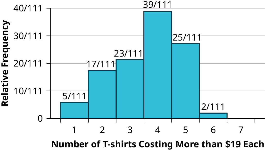


Figure 2.24図 2.24
Exercise 28問題 28
The percentage of people who own at most three T-shirts costing more than $19 each is approximately:
1枚19ドルを超えるTシャツの所有枚数が3枚以下の人の百分率は、およそ次のどれか。
- 21
- 59
- 41
- Cannot be determined判断できない
Solution解き方
c
Exercise 29問題 29
If the data were collected by asking the first 111 people who entered the store, then the type of sampling is:
入店した最初の111人に尋ねてデータを集めたなら、抽出法は次のどれか。
- cluster集落抽出
- simple random単純無作為抽出
- stratified層化抽出
- convenience便宜抽出
Exercise 30問題 30
Following are the rates of unmarried adults for the 50 U.S. states and Washington, DC.
以下は、米国50州とワシントンDCの未婚成人の割合である。
State 州 |
Percent (%) 百分率(%) |
State 州 |
Percent (%) 百分率(%) |
State 州 |
Percent (%) 百分率(%) |
|---|---|---|---|---|---|
Alabama アラバマ |
32.2 |
Kentucky ケンタッキー |
31.3 |
North Dakota ノースダコタ |
27.2 |
Alaska アラスカ |
24.5 |
Louisiana ルイジアナ |
31.0 |
Ohio オハイオ |
29.2 |
Arizona アリゾナ |
24.3 |
Maine メイン |
26.8 |
Oklahoma オクラホマ |
30.4 |
Arkansas アーカンソー |
30.1 |
Maryland メリーランド |
27.1 |
Oregon オレゴン |
26.8 |
California カリフォルニア |
24.0 |
Massachusetts マサチューセッツ |
23.0 |
Pennsylvania ペンシルベニア |
28.6 |
Colorado コロラド |
21.0 |
Michigan ミシガン |
30.9 |
Rhode Island ロードアイランド |
25.5 |
Connecticut コネチカット |
22.5 |
Minnesota ミネソタ |
24.8 |
South Carolina サウスカロライナ |
31.5 |
Delaware デラウェア |
28.0 |
Mississippi ミシシッピ |
34.0 |
South Dakota サウスダコタ |
27.3 |
Washington, DC ワシントンDC |
22.2 |
Missouri ミズーリ |
30.5 |
Tennessee テネシー |
30.8 |
Florida フロリダ |
26.6 |
Montana モンタナ |
23.0 |
Texas テキサス |
31.0 |
Georgia ジョージア |
29.6 |
Nebraska ネブラスカ |
26.9 |
Utah ユタ |
22.5 |
Hawaii ハワイ |
22.7 |
Nevada ネバダ |
22.4 |
Vermont バーモント |
23.2 |
Idaho アイダホ |
26.5 |
New Hampshire ニューハンプシャー |
25.0 |
Virginia ヴァージニア |
26.0 |
Illinois イリノイ |
28.2 |
New Jersey ニュージャージー |
23.8 |
Washington ワシントン |
25.5 |
Indiana インディアナ |
29.6 |
New Mexico ニューメキシコ |
25.1 |
West Virginia ウェストヴァージニア |
32.5 |
Iowa アイオワ |
28.4 |
New York ニューヨーク |
23.9 |
Wisconsin ウィスコンシン |
26.3 |
Kansas カンザス |
29.4 |
North Carolina ノースカロライナ |
27.8 |
Wyoming ワイオミング |
25.1 |
Construct a bar graph of the unmarried adult rates of your state and the four states closest to your state. Hint: Label the x-axis with the states.
自分の州と、それに最も近い4州の未婚成人の割合を棒グラフにせよ。ヒント:x軸に州名を付ける。
Solution解き方
Answers will vary.
答えはさまざまである。
Frequency
度数
the number of times a value of the data occurs
あるデータの値が現れる回数。
Histogram
ヒストグラム
a graphical representation in x-y form of the distribution of data in a data set; x represents the data and y represents the frequency, or relative frequency. The graph consists of contiguous rectangles.
データセットの分布をx-y形式で図示したもの。xはデータ、yは度数または相対度数を表す。互いに接する長方形からなる。
Relative Frequency
相対度数
the ratio of the number of times a value of the data occurs in the set of all outcomes to the number of all outcomes
すべての結果の中で、あるデータの値が現れる回数を、結果の総数で割った比。