第3章微分
3.2 The Derivative as a Function3.2 関数としての導関数
Learning Objectives学習目標
- Define the derivative function of a given function.与えられた関数の導関数を定義する。
- Graph a derivative function from the graph of a given function.与えられた関数のグラフから、導関数のグラフを描く。
- State the connection between derivatives and continuity.微分可能性と連続性のつながりを述べる。
- Describe three conditions for when a function does not have a derivative.関数が微分できない三つの状況を説明する。
- Explain the meaning of a higher-order derivative.高階導関数の意味を説明する。
As we have seen, the derivative of a function at a given point gives us the rate of change or slope of the tangent line to the function at that point. If we differentiate a position function at a given time, we obtain the velocity at that time. It seems reasonable to conclude that knowing the derivative of the function at every point would produce valuable information about the behavior of the function. However, the process of finding the derivative at even a handful of values using the techniques of the preceding section would quickly become quite tedious. In this section we define the derivative function and learn a process for finding it.
英語のヒント
これまで見たように、ある点での関数の微分係数は、その点における変化率、あるいは接線の傾きを表す。時刻を指定して位置関数を微分すれば、その時刻の速度が得られる。すべての点で微分係数が分かれば、関数の振る舞いについて価値ある情報が得られる、と考えるのは自然である。しかし前節の方法で、ほんの数個の値について微分係数を求めるだけでも、すぐにかなり面倒になる。この節では導関数を定義し、それを求める手順を学ぶ。
Derivative Functions導関数
The derivative function gives the derivative of a function at each point in the domain of the original function for which the derivative is defined. We can formally define a derivative function as follows.
英語のヒント
導関数は、もとの関数の定義域のうち微分係数が定義される各点に対して、その点での微分係数を与える関数である。厳密には、次のように定義する。
A function is said to be differentiable at if exists. More generally, a function is said to be differentiable on if it is differentiable at every point in an open set and a differentiable function is one in which exists on its domain.
英語のヒント
関数は、が存在するとき、で微分可能であるという。より一般に、開集合のすべての点で微分可能な関数を、上で微分可能という。また、定義域の全体でが存在する関数を、微分可能な関数という。
In the next few examples we use Equation 3.9 to find the derivative of a function.
次のいくつかの例題では、式3.9を使って導関数を求める。
Example 3.11例題 3.11
Finding the Derivative of a Square-Root Function平方根の関数の導関数を求める
Find the derivative of
の導関数を求めなさい。
Solution解き方
Start directly with the definition of the derivative function. Use Equation 3.1.
導関数の定義から直接計算する。原文は式3.1を参照しているが、ここで実際に用いる導関数の定義は式3.9である。
Example 3.12例題 3.12
Finding the Derivative of a Quadratic Function二次関数の導関数を求める
Find the derivative of the function
関数の導関数を求めなさい。
Solution解き方
Follow the same procedure here, but without having to multiply by the conjugate.
同じ手順で進めればよいが、ここでは共役な式を掛ける必要はない。
We use a variety of different notations to express the derivative of a function. In Example 3.12 we showed that if then If we had expressed this function in the form we could have expressed the derivative as or We could have conveyed the same information by writing Thus, for the function each of the following notations represents the derivative of
英語のヒント
導関数を表すには、さまざまな記法を使う。例題3.12では、ならであることを示した。この関数をという形で書いていたなら、導関数はまたはと表せた。同じ内容をと書いてもよい。したがって、関数について、次の記法はいずれもの導関数を表す。
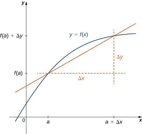
In place of we may also use Use of the notation (called Leibniz notation) is quite common in engineering and physics. To understand this notation better, recall that the derivative of a function at a point is the limit of the slopes of secant lines as the secant lines approach the tangent line. The slopes of these secant lines are often expressed in the form where is the difference in the values corresponding to the difference in the values, which are expressed as (Figure 3.11). Thus the derivative, which can be thought of as the instantaneous rate of change of with respect to is expressed as
英語のヒント
の代わりにと書くこともできる。という記法はライプニッツの記法と呼ばれ、工学や物理学で広く使われる。この記法を理解するため、ある点の微分係数が、割線を接線に近づけたときの傾きの極限であることを思い出そう。割線の傾きは、しばしばの形で表す。の値の差をと書き、それに対応するの値の差をと書く(図3.11)。したがって、に対するの瞬間変化率と考えられる微分係数は、次のように表される。
OpenStax, Rice University; Calculus Volume 1. · CC BY-NC-SA 4.0
Figure 3.11図 3.11
The derivative is expressed as
微分係数はと表される。
Graphing a Derivative導関数のグラフ
We have already discussed how to graph a function, so given the equation of a function or the equation of a derivative function, we could graph it. Given both, we would expect to see a correspondence between the graphs of these two functions, since gives the rate of change of a function (or slope of the tangent line to
英語のヒント
関数のグラフの描き方はすでに学んだので、関数の式や導関数の式が与えられれば、そのグラフを描ける。両方の式があれば、二つのグラフの間には対応があるはずである。なぜなら、は関数の変化率、すなわちの接線の傾きを与えるからである。
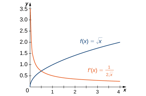
In Example 3.11 we found that for If we graph these functions on the same axes, as in Figure 3.12, we can use the graphs to understand the relationship between these two functions. First, we notice that is increasing over its entire domain, which means that the slopes of its tangent lines at all points are positive. Consequently, we expect for all values of in its domain. Furthermore, as increases, the slopes of the tangent lines to are decreasing and we expect to see a corresponding decrease in We also observe that is undefined and that corresponding to a vertical tangent to at
英語のヒント
OpenStax, Rice University; Calculus Volume 1. · CC BY-NC-SA 4.0
Figure 3.12図 3.12
The derivative is positive everywhere because the function is increasing.
関数が増加しているため、導関数はその定義域全体で正になる。
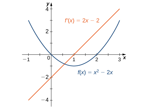
In Example 3.12 we found that for The graphs of these functions are shown in Figure 3.13. Observe that is decreasing for For these same values of For values of is increasing and Also, has a horizontal tangent at and
OpenStax, Rice University; Calculus Volume 1. · CC BY-NC-SA 4.0
Figure 3.13図 3.13
The derivative where the function is decreasing and where is increasing. The derivative is zero where the function has a horizontal tangent.
関数が減少するところでは、が増加するところではとなる。関数が水平な接線をもつところでは、導関数の値は0になる。
Example 3.13例題 3.13
Sketching a Derivative Using a Function関数のグラフから導関数の概形を描く
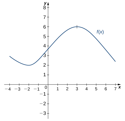
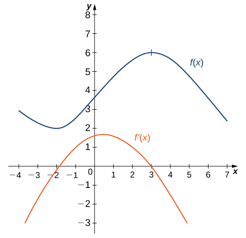
Use the following graph of to sketch a graph of
次ののグラフから、のグラフの概形を描きなさい。
OpenStax, Rice University; Calculus Volume 1. · CC BY-NC-SA 4.0
Solution解き方
The solution is shown in the following graph. Observe that is increasing and on Also, is decreasing and on and on Also note that has horizontal tangents at and and and
解答を次のグラフに示す。ではが増加し、となる。およびでは、が減少し、となる。また、はとで水平な接線をもち、、である。
OpenStax, Rice University; Calculus Volume 1. · CC BY-NC-SA 4.0