第3章微分
3.1 Defining the Derivative3.1 微分係数の定義
Learning Objectives学習目標
- Recognize the meaning of the tangent to a curve at a point.曲線上のある点における接線の意味を理解する。
- Calculate the slope of a tangent line.接線の傾きを計算する。
- Identify the derivative as the limit of a difference quotient.微分係数を、差商の極限として捉える。
- Calculate the derivative of a given function at a point.与えられた関数の、ある点における微分係数を計算する。
- Describe the velocity as a rate of change.速度を変化率として説明する。
- Explain the difference between average velocity and instantaneous velocity.平均速度と瞬間速度の違いを説明する。
- Estimate the derivative from a table of values.値の表から微分係数を推定する。
Now that we have both a conceptual understanding of a limit and the practical ability to compute limits, we have established the foundation for our study of calculus, the branch of mathematics in which we compute derivatives and integrals. Most mathematicians and historians agree that calculus was developed independently by the Englishman Isaac Newton and the German Gottfried Leibniz whose images appear in Figure 3.2. When we credit Newton and Leibniz with developing calculus, we are really referring to the fact that Newton and Leibniz were the first to understand the relationship between the derivative and the integral. Both mathematicians benefited from the work of predecessors, such as Barrow, Fermat, and Cavalieri. The initial relationship between the two mathematicians appears to have been amicable; however, in later years a bitter controversy erupted over whose work took precedence. Although it seems likely that Newton did, indeed, arrive at the ideas behind calculus first, we are indebted to Leibniz for the notation that we commonly use today.
英語のヒント
極限の概念を理解し、実際に極限を計算する力も身につけたので、導関数と積分を求める数学の分野である微積分を学ぶ土台ができた。微積分は、イングランドのアイザック・ニュートンとドイツのゴットフリート・ライプニッツが独立に発展させた、という見方で数学者や歴史家の大半は一致している。両者の肖像を図3.2に示す。ニュートンとライプニッツを微積分の創始者として評価するとき、実際に指しているのは、微分と積分の関係を最初に理解したのがこの二人だったという事実である。二人とも、バロー、フェルマー、カヴァリエリなど、先人の仕事から恩恵を受けていた。二人の関係は、当初は友好的だったようである。しかし後年、どちらの仕事が先だったかをめぐって激しい論争が起こった。微積分の基礎にある考えに最初に達したのは、おそらく実際にニュートンだったと考えられる。それでも、現在よく使う記法についてはライプニッツに負うところが大きい。

OpenStax, Rice University; Calculus Volume 1. · CC BY-NC-SA 4.0
Figure 3.2図 3.2
Newton and Leibniz are credited with developing calculus independently.
ニュートンとライプニッツは、それぞれ独立に微積分を発展させたと評価されている。
Tangent Lines接線
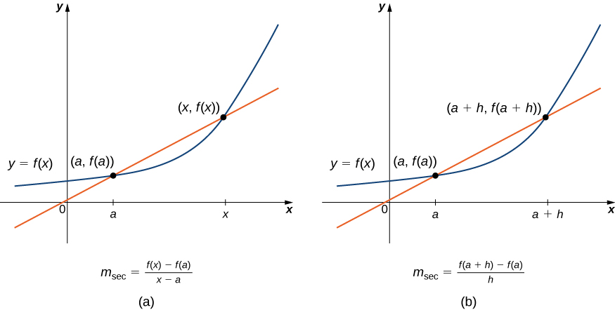
We begin our study of calculus by revisiting the notion of secant lines and tangent lines. Recall that we used the slope of a secant line to a function at a point to estimate the rate of change, or the rate at which one variable changes in relation to another variable. We can obtain the slope of the secant by choosing a value of near and drawing a line through the points and as shown in Figure 3.3. The slope of this line is given by an equation in the form of a difference quotient:
英語のヒント
微積分の学習を、割線と接線の考えを振り返ることから始めよう。関数のグラフ上の点を通る割線の傾きを用い、変化率、すなわち一方の変数がもう一方の変数に対して変わる割合を推定したことを思い出そう。図3.3のように、の値をの近くに選び、点とを通る直線を引けば、割線の傾きが得られる。この直線の傾きは、次の差商の形の式で与えられる。
We can also calculate the slope of a secant line to a function at a value a by using this equation and replacing with where is a value close to 0. We can then calculate the slope of the line through the points and In this case, we find the secant line has a slope given by the following difference quotient with increment
英語のヒント
同じ式でをに置き換えても、値aにおける割線の傾きを計算できる。ここでは0に近い値である。点とを通る直線の傾きを求めると、この場合は、増分を用いた次の差商で表される。
These two expressions for calculating the slope of a secant line are illustrated in Figure 3.3. We will see that each of these two methods for finding the slope of a secant line is of value. Depending on the setting, we can choose one or the other. The primary consideration in our choice usually depends on ease of calculation.
英語のヒント
割線の傾きを計算する二つの式を図3.3に示す。どちらの方法にも、それぞれ使いどころがある。状況に応じて、どちらかを選べばよい。通常、選ぶ際の主な判断基準は、計算しやすいかどうかである。
OpenStax, Rice University; Calculus Volume 1. · CC BY-NC-SA 4.0
Figure 3.3図 3.3
We can calculate the slope of a secant line in either of two ways.
割線の傾きは、二通りの方法で計算できる。
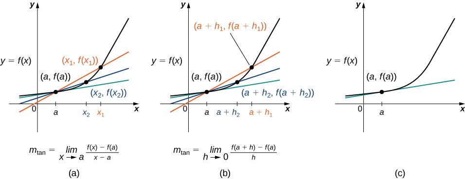
In Figure 3.4(a) we see that, as the values of approach the slopes of the secant lines provide better estimates of the rate of change of the function at Furthermore, the secant lines themselves approach the tangent line to the function at which represents the limit of the secant lines. Similarly, Figure 3.4(b) shows that as the values of get closer to the secant lines also approach the tangent line. The slope of the tangent line at is the rate of change of the function at as shown in Figure 3.4(c).
英語のヒント
OpenStax, Rice University; Calculus Volume 1. · CC BY-NC-SA 4.0
Figure 3.4図 3.4
The secant lines approach the tangent line (shown in green) as the second point approaches the first.
2点目が1点目に近づくと、割線は緑色で示した接線に近づく。
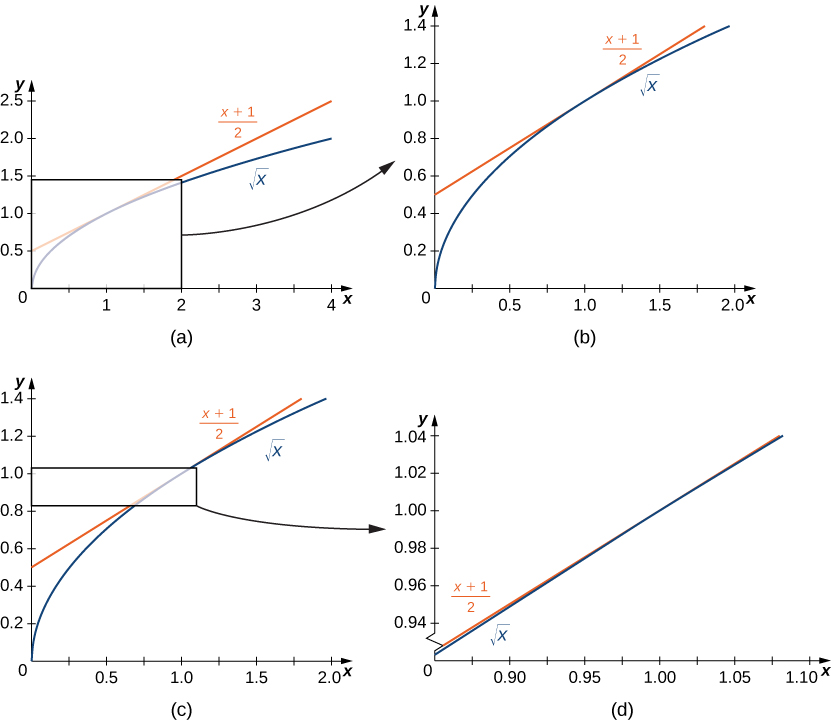
In Figure 3.5 we show the graph of and its tangent line at in a series of tighter intervals about As the intervals become narrower, the graph of the function and its tangent line appear to coincide, making the values on the tangent line a good approximation to the values of the function for choices of close to In fact, the graph of itself appears to be locally linear in the immediate vicinity of
英語のヒント
図3.5では、のグラフとにおける接線を、のまわりの区間を次第に狭めながら示している。区間が狭くなるにつれ、関数のグラフと接線は重なって見えるようになる。このため、をに近く選ぶと、接線上の値は関数値のよい近似となる。実際、のグラフ自体が、のごく近くでは直線のように見える。
OpenStax, Rice University; Calculus Volume 1. · CC BY-NC-SA 4.0
Figure 3.5図 3.5
For values of close to the graph of and its tangent line appear to coincide.
の値がに近いと、のグラフと接線は重なって見える。
Formally we may define the tangent line to the graph of a function as follows.
関数のグラフの接線を、厳密には次のように定義できる。
Just as we have used two different expressions to define the slope of a secant line, we use two different forms to define the slope of the tangent line. In this text we use both forms of the definition. As before, the choice of definition will depend on the setting. Now that we have formally defined a tangent line to a function at a point, we can use this definition to find equations of tangent lines.
英語のヒント
割線の傾きを二通りの式で定義したのと同じように、接線の傾きも二通りの形で定義する。この本では、両方の定義を使う。先ほどと同様に、どちらを選ぶかは状況による。ある点における関数の接線を厳密に定義できたので、この定義を使って接線の方程式を求められる。
Example 3.1例題 3.1
Finding a Tangent Line接線を求める
Find the equation of the line tangent to the graph of at
のグラフの、における接線の方程式を求めなさい。
Solution解き方
First find the slope of the tangent line. In this example, use Equation 3.3.
まず接線の傾きを求める。この例では式3.3を使う。
Next, find a point on the tangent line. Since the line is tangent to the graph of at it passes through the point We have so the tangent line passes through the point
次に、接線上の1点を求める。この直線はでのグラフに接するので、点を通る。だから、接線は点を通る。
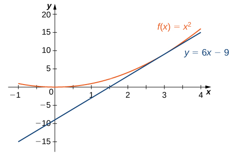
Using the point-slope equation of the line with the slope and the point we obtain the line Simplifying, we have The graph of and its tangent line at are shown in Figure 3.6.
傾き、通る点を用いて、直線の点傾き形式の方程式を書くととなる。整理するとが得られる。のグラフと、における接線を図3.6に示す。
OpenStax, Rice University; Calculus Volume 1. · CC BY-NC-SA 4.0
Figure 3.6図 3.6
The tangent line to at
のにおける接線。
Example 3.2例題 3.2
The Slope of a Tangent Line Revisited接線の傾きを別の定義から求める
Use Equation 3.4 to find the slope of the line tangent to the graph of at
式3.4を使い、のグラフのにおける接線の傾きを求めなさい。
Solution解き方
The steps are very similar to Example 3.1. See Equation 3.4 for the definition.
We obtained the same value for the slope of the tangent line by using the other definition, demonstrating that the formulas can be interchanged.
英語のヒント
もう一方の定義を使っても、接線の傾きは同じ値になった。このことは、二つの公式を置き換えて使えることを示している。
Example 3.3例題 3.3
Finding the Equation of a Tangent Line接線の方程式を求める
Find the equation of the line tangent to the graph of at
のグラフの、における接線の方程式を求めなさい。
Solution解き方
We can use Equation 3.3, but as we have seen, the results are the same if we use Equation 3.4.
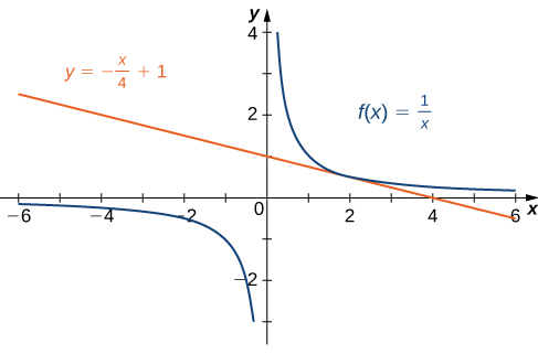
We now know that the slope of the tangent line is To find the equation of the tangent line, we also need a point on the line. We know that Since the tangent line passes through the point we can use the point-slope equation of a line to find the equation of the tangent line. Thus the tangent line has the equation The graphs of and are shown in Figure 3.7.
接線の傾きはだと分かった。接線の方程式を求めるには、直線上の1点も必要である。であり、接線は点を通る。したがって、直線の点傾き形式の方程式から接線の方程式を求められる。得られる式はである。とのグラフを図3.7に示す。
OpenStax, Rice University; Calculus Volume 1. · CC BY-NC-SA 4.0
Figure 3.7図 3.7
The line is tangent to at
直線は、でに接している。