第12章線形回帰と相関
12.3 The Regression Equation12.3 回帰方程式
Data rarely fit a straight line exactly. Usually, you must be satisfied with rough predictions. Typically, you have a set of data whose scatter plot appears to "fit" a straight line. This is called a Line of Best Fit or Least-Squares Line.
英語のヒント
データが直線に完全に一致することはめったにない。通常は、おおまかな予測で満足しなければならない。一般には、散布図が直線に「適合」して見えるデータ集合を扱う。この直線を最適な当てはめ直線、または最小二乗直線という。
Collaborative Exercise共同演習
Example 12.6例題 12.6
A random sample of 11 statistics students produced the following data, where x is the third exam score out of 80, and y is the final exam score out of 200. Can you predict the final exam score of a random student if you know the third exam score?
統計学を学ぶ学生11人を無作為に抽出し、次のデータが得られた。xは80点満点の第3回試験の得点、yは200点満点の期末試験の得点である。ある学生の第3回試験の得点が分かれば、期末試験の得点を予測できるだろうか。
x (third exam score) x(第3回試験の得点) |
y (final exam score) y(期末試験の得点) |
|---|---|
65 |
175 |
67 |
133 |
71 |
185 |
71 |
163 |
66 |
126 |
75 |
198 |
67 |
153 |
70 |
163 |
71 |
159 |
69 |
151 |
69 |
159 |
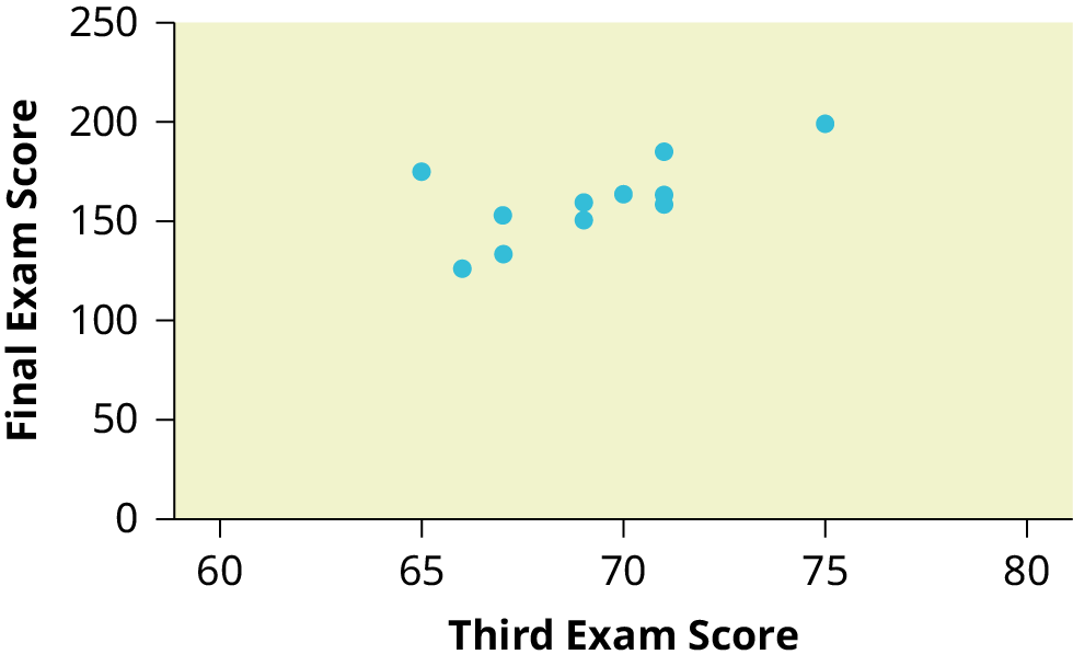
Figure 12.15図 12.15
Scatter plot showing the scores on the final exam based on scores from the third exam.
第3回試験の得点に対応する期末試験の得点を示す散布図。
The third exam score, x, is the independent variable and the final exam score, y, is the dependent variable. We will plot a regression line that best "fits" the data. If each of you were to fit a line "by eye," you would draw different lines. We can use what is called a least-squares regression line to obtain the best fit line.
英語のヒント
第3回試験の得点xが独立変数、期末試験の得点yが従属変数である。データに最もよく「適合」する回帰直線を描こう。各自が「目分量」で直線を当てはめると、異なる直線になるだろう。最適な直線を得るために、最小二乗回帰直線と呼ばれるものを使える。
Consider the following diagram. Each point of data is of the the form (x, y) and each point of the line of best fit using least-squares linear regression has the form (x, ŷ).
次の図を考えよう。各データ点は(x, y)という形をとり、最小二乗線形回帰による最適直線上の各点は(x, ŷ)という形をとる。
The ŷ is read "y hat" and is the estimated value of y. It is the value of y obtained using the regression line. It is not generally equal to y from data.
ŷは「ワイハット」と読み、yの推定値を表す。回帰直線を使って得られるyの値であり、一般にデータのyとは等しくない。
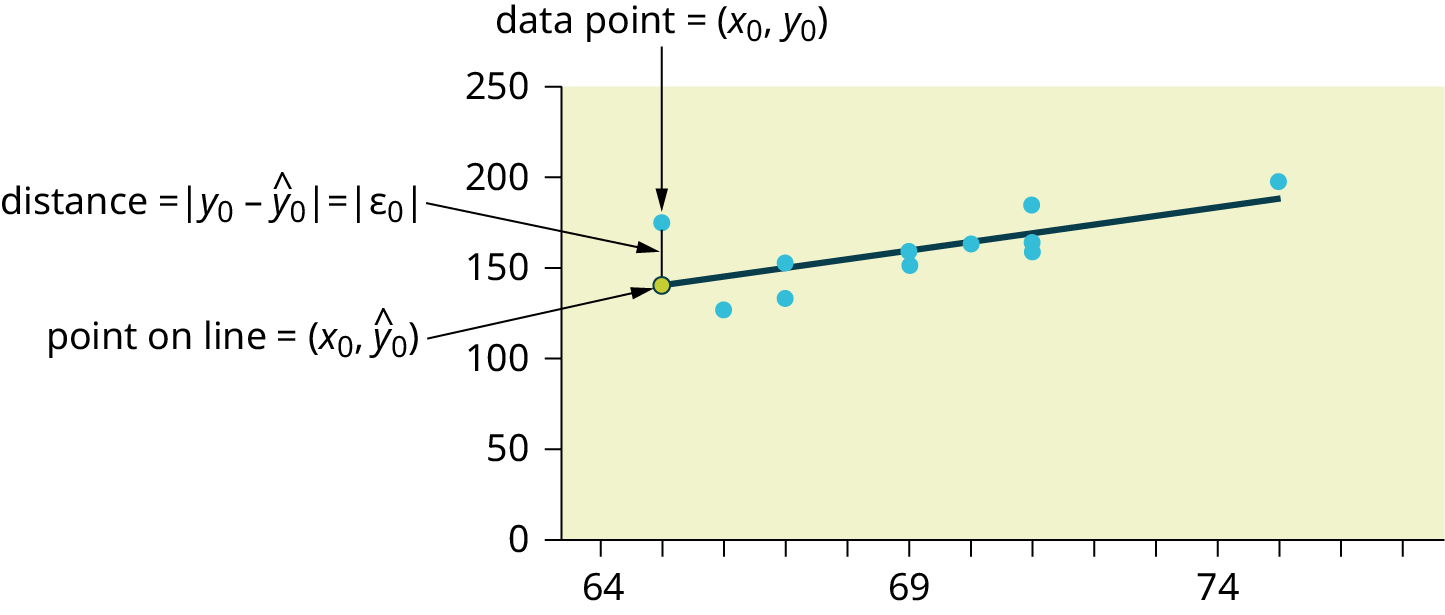


Figure 12.16図 12.16
The term y0 – ŷ0 = ε0 is called the "error" or residual. It is not an error in the sense of a mistake. The absolute value of a residual measures the vertical distance between the actual value of y and the estimated value of y. In other words, it measures the vertical distance between the actual data point and the predicted point on the line.
英語のヒント
y0 − ŷ0 = ε0を「誤差」または残差という。ここでの誤差は、間違いという意味ではない。残差の絶対値は、yの実際の値と推定値の間の垂直距離を測る。言い換えると、実際のデータ点と、直線上の予測点との垂直距離である。
If the observed data point lies above the line, the residual is positive, and the line underestimates the actual data value for y. If the observed data point lies below the line, the residual is negative, and the line overestimates that actual data value for y.
英語のヒント
観測されたデータ点が直線より上にあれば、残差は正であり、直線はyの実際の値を過小評価する。点が直線より下にあれば、残差は負であり、直線はyの実際の値を過大評価する。
In the diagram in Figure 12.16, y0 – ŷ0 = ε0 is the residual for the point shown. Here the point lies above the line and the residual is positive.
図12.16では、y0 − ŷ0 = ε0が、示された点の残差である。ここでは点が直線より上にあり、残差は正である。
ε = the Greek letter epsilon
ε = ギリシャ文字のイプシロン
For each data point, you can calculate the residuals or errors, yi - ŷi = εi for i = 1, 2, 3, ..., 11.
各データ点について、i = 1, 2, 3, ..., 11として、残差または誤差yi − ŷi = εiを計算できる。
Each |ε| is a vertical distance.
各|ε|は垂直距離である。
For the example about the third exam scores and the final exam scores for the 11 statistics students, there are 11 data points. Therefore, there are 11 ε values. If you square each ε and add, you get
統計学を学ぶ学生11人の第3回試験と期末試験の例では、データ点が11個ある。したがって、εの値も11個ある。各εを二乗して足し合わせると、次のようになる。
This is called the Sum of Squared Errors (SSE).
これを誤差平方和(SSE)という。
Using calculus, you can determine the values of a and b that make the SSE a minimum. When you make the SSE a minimum, you have determined the points that are on the line of best fit. It turns out that the line of best fit has the equation:
英語のヒント
微積分を用いると、SSEを最小にするaとbの値を決められる。SSEを最小にすると、最適な当てはめ直線上の点が定まる。この直線の方程式は、次のようになる。
where and .
ここで、、である。
The sample means of the x values and the y values are and , respectively. The best fit line always passes through the point .
英語のヒント
xの値とyの値の標本平均は、それぞれとである。最適な当てはめ直線は、必ず点を通る。
The slope b can be written as where sy = the standard deviation of the y values and sx = the standard deviation of the x values. r is the correlation coefficient, which is discussed in the next section.
傾きbはと書ける。ここでsyはyの値の標準偏差、sxはxの値の標準偏差である。rは相関係数で、次の節で論じる。