第12章線形回帰と相関

Numerical Identification of Outliers数値による外れ値の特定

In Table 12.20, the first two columns are the third-exam and final-exam data. The third column shows the predicted ŷ values calculated from the line of best fit: ŷ = –173.5 + 4.83x. The residuals, or errors, have been calculated in the fourth column of the table: observed y value−predicted y value = y − ŷ.

表12.20の最初の2列は、第3回試験と期末試験のデータである。第3列は、最適直線ŷ = −173.5 + 4.83xから計算した予測値ŷを示す。第4列では残差、すなわち誤差を、観測されたy − 予測されたy = y − ŷとして計算している。

s is the standard deviation of all the y − ŷ = ε values where n = the total number of data points. If each residual is calculated and squared, and the results are added, we get the SSE. The standard deviation of the residuals is calculated from the SSE as:

sは、すべてのy − ŷ = εの値の標準偏差であり、nはデータ点の総数である。各残差を計算して二乗し、足し合わせるとSSEが得られる。残差の標準偏差は、SSEから次のように計算する。

s = \sqrt{\frac{S S E}{n - 2}}

Rather than calculate the value of s ourselves, we can find s using the computer or calculator. For this example, the calculator function LinRegTTest found s = 16.4 as the standard deviation of the residuals

sを自分で計算する代わりに、コンピューターや電卓で求められる。この例では、電卓のLinRegTTestが、残差の標準偏差としてs = 16.4を与えた。

35
–17
16
–6
–19
9
3
–1
–10
–9
–1

Table 12.20表 12.20
x	y	ŷ	y – ŷ y − ŷ
65	175	140	175 – 140 = 35
67	133	150	133 – 150= –17
71	185	169	185 – 169 = 16
71	163	169	163 – 169 = –6
66	126	145	126 – 145 = –19
75	198	189	198 – 189 = 9
67	153	150	153 – 150 = 3
70	163	164	163 – 164 = –1
71	159	169	159 – 169 = –10
69	151	160	151 – 160 = –9
69	159	160	159 – 160 = –1

We are looking for all data points for which the residual is greater than 2s = 2(16.4) = 32.8 or less than –32.8. Compare these values to the residuals in column four of the table. The only such data point is the student who had a grade of 65 on the third exam and 175 on the final exam; the residual for this student is 35.

残差が2s = 2(16.4) = 32.8より大きいか、−32.8より小さいデータ点をすべて探している。この値を表の第4列の残差と比較しよう。該当するのは、第3回試験が65点、期末試験が175点だった学生の点だけで、残差は35である。

How does the outlier affect the best fit line?外れ値は最適直線にどう影響するか

Numerically and graphically, we have identified the point (65, 175) as an outlier. We should re-examine the data for this point to see if there are any problems with the data. If there is an error, we should fix the error if possible, or delete the data. If the data is correct, we would leave it in the data set. For this problem, we will suppose that we examined the data and found that this outlier data was an error. Therefore we will continue on and delete the outlier, so that we can explore how it affects the results, as a learning experience.

数値とグラフから、点(65, 175)を外れ値と特定した。この点のデータを再確認し、問題がないか調べるべきである。誤りがあれば可能な限り修正し、そうでなければ削除する。正しいデータなら、集合に残す。この問題では、調べた結果、この外れ値のデータに誤りがあったと仮定する。そこで削除し、学習のため、結果にどのような影響があるかを調べる。

Compute a new best-fit line and correlation coefficient using the ten remaining points:残る10点を使い、新しい最適直線と相関係数を計算する

On the TI-83, TI-83+, TI-84+ calculators, delete the outlier from L1 and L2. Using the LinRegTTest, the new line of best fit and the correlation coefficient are:

TI-83、TI-83+、TI-84+電卓で、L1とL2から外れ値を削除する。LinRegTTestを使うと、新しい最適直線と相関係数は次のようになる。

ŷ = –355.19 + 7.39x and r = 0.9121

ŷ = −355.19 + 7.39x、r = 0.9121

The new line with r = 0.9121 is a stronger correlation than the original (r = 0.6631) because r = 0.9121 is closer to one. This means that the new line is a better fit to the ten remaining data values. The line can better predict the final exam score given the third exam score.

新しい直線のr = 0.9121は元のr = 0.6631より1に近いため、相関が強い。つまり、新しい直線は残る10個の値によりよく適合する。第3回試験の得点から、期末試験の得点をよりよく予測できる。

Numerical Identification of Outliers: Calculating s and Finding Outliers Manually数値による外れ値の特定：sを計算し、手計算で外れ値を求める

If you do not have the function LinRegTTest, then you can calculate the outlier in the first example by doing the following.

First, square each |y – ŷ|

LinRegTTest機能がない場合は、次の手順で最初の例の外れ値を求められる。まず、各|y − ŷ|を二乗する。

The squares are

二乗した値は、

35²
17²
16²
6²
19²
9²
3²
1²
10²
9²
1²

Then, add (sum) all the |y – ŷ| squared terms using the formula

次に、次の式を使って、|y − ŷ|を二乗した項をすべて足し合わせる。

\overset{11}{\underset{i = 1}{Σ}} {(| y_{i} - {\hat{y}}_{i} |)}^{2} = \overset{11}{\underset{i = 1}{Σ}} ε_{i}^{2}

(Recall that y_i – ŷ_i = ε_i.)

\overset{11}{\underset{i = 1}{Σ}} {(| y_{i} - {\hat{y}}_{i} |)}^{2} = \overset{11}{\underset{i = 1}{Σ}} ε_{i}^{2}

（y_i − ŷ_i = ε_iであることを思い出そう。）

= 35² + 17² + 16² + 6² + 19² + 9² + 3² + 1² + 10² + 9² + 1²

= 2440 = SSE. The result, SSE is the Sum of Squared Errors.

= 2440 = SSE。結果のSSEは誤差平方和である。

Next, calculate s, the standard deviation of all the y – ŷ = ε values where n = the total number of data points.

次に、すべてのy − ŷ = εの値の標準偏差sを求める。nはデータ点の総数である。

The calculation is

s = \sqrt{\frac{SSE}{n - 2}}

計算式は

s = \sqrt{\frac{SSE}{n - 2}}

である。

For the third exam/final exam problem,

s = \sqrt{\frac{2440}{11 - 2}} = 16.47

第3回試験と期末試験の問題では、

s = \sqrt{\frac{2440}{11 - 2}} = 16.47

となる。

Next, multiply s by 2:
(2)(16.47) = 32.94
32.94 is 2 standard deviations away from the mean of the y – ŷ values.

次にsを2倍する：(2)(16.47) = 32.94。この32.94は、y − ŷの平均から標準偏差の2倍離れた距離である。

If we were to measure the vertical distance from any data point to the corresponding point on the line of best fit and that distance is at least 2s, then we would consider the data point to be "too far" from the line of best fit. We call that point a potential outlier.

データ点と、最適直線上の対応する点の垂直距離を測り、その距離が少なくとも2sなら、点は直線から「遠すぎる」とみなす。この点を外れ値の候補と呼ぶ。

For the example, if any of the |y – ŷ| values are at least 32.94, the corresponding (x, y) data point is a potential outlier.

この例で|y − ŷ|が少なくとも32.94となる値があれば、それに対応する(x, y)のデータ点は外れ値の候補である。

For the third exam/final exam problem, all the |y – ŷ|'s are less than 31.29 except for the first one which is 35.

第3回試験と期末試験の問題では、最初の35を除き、すべての|y − ŷ|が31.29未満である。

35 > 31.29 That is, |y – ŷ| ≥ (2)(s)

35 > 31.29、すなわち|y − ŷ| ≥ (2)(s)。

The point which corresponds to |y – ŷ| = 35 is (65, 175). Therefore, the data point (65,175) is a potential outlier. For this example, we will delete it. (Remember, we do not always delete an outlier.)

|y − ŷ| = 35に対応する点は(65, 175)である。したがって、点(65, 175)は外れ値の候補である。この例では削除する。（外れ値をいつも削除するわけではないことを覚えておこう。）

The next step is to compute a new best-fit line using the ten remaining points. The new line of best fit and the correlation coefficient are:

次に、残る10点で新しい最適直線を計算する。新しい直線と相関係数は次のとおりである。

ŷ = –355.19 + 7.39x and r = 0.9121

ŷ = −355.19 + 7.39x、r = 0.9121

Example 12.13例題 12.13

Using this new line of best fit (based on the remaining ten data points in the third exam/final exam example), what would a student who receives a 73 on the third exam expect to receive on the final exam? Is this the same as the prediction made using the original line?

この新しい最適直線（「第3回試験と期末試験の例」の残る10点に基づく）を使うと、第3回試験が73点の学生は、期末試験で何点を取ると期待されるか。元の直線を使った予測と同じか。

Solution解き方

Using the new line of best fit, ŷ = –355.19 + 7.39(73) = 184.28. A student who scored 73 points on the third exam would expect to earn 184 points on the final exam.

The original line predicted ŷ = –173.51 + 4.83(73) = 179.08 so the prediction using the new line with the outlier eliminated differs from the original prediction.

新しい直線では、ŷ = −355.19 + 7.39(73) = 184.28となる。第3回試験が73点の学生は、期末試験で184点を取ると期待される。元の直線の予測はŷ = −173.51 + 4.83(73) = 179.08だったので、外れ値を除いた新しい直線の予測は、元の予測と異なる。

Example 12.14例題 12.14

The Consumer Price Index (CPI) measures the average change over time in the prices paid by urban consumers for consumer goods and services. The CPI affects nearly all Americans because of the many ways it is used. One of its biggest uses is as a measure of inflation. By providing information about price changes in the Nation's economy to government, business, and labor, the CPI helps them to make economic decisions. The President, Congress, and the Federal Reserve Board use the CPI's trends to formulate monetary and fiscal policies. In the following table, x is the year and y is the CPI.

英語のヒント

消費者物価指数（CPI）は、都市の消費者が消費財やサービスに支払う価格の、時間的な平均変化を測る。多様な用途があるため、ほぼすべての米国人に影響する。最も大きな用途の一つは、インフレの指標である。CPIは政府、企業、労働者に国内経済の価格変化の情報を提供し、経済的な意思決定を助ける。大統領、議会、連邦準備制度理事会は、CPIの傾向を使って金融・財政政策を策定する。次の表では、xは年、yはCPIである。

Dataデータ

Table 12.21表 12.21
x	y	x	y
1915	10.1	1979	72.6
1926	17.7	1980	82.4
1935	13.7	1986	109.6
1940	14.7	1991	130.7
1947	24.1	1999	166.6
1952	26.5	2010	219.2
1964	31.0	2020	258
1969	36.7	2023	299.2
1975	49.3

Draw a scatterplot of the data.
データの散布図を描こう。
Calculate the least squares line. Write the equation in the form ŷ = a + bx.
最小二乗直線を計算し、ŷ = a + bxの形で方程式を書こう。
Draw the line on the scatterplot.
散布図に直線を描こう。
Find the correlation coefficient. Is it significant?
相関係数を求めよう。有意か。
What is the average CPI for the year 1990?
1990年の平均CPIはいくつか。

Solution解き方

See Figure 12.29.
図12.29を参照。
ŷ = –3204 + 1.662x is the equation of the line of best fit.
最適な当てはめ直線の方程式は、ŷ = −3204 + 1.662xである。
r = 0.8694
The number of data points is n = 14. Use the 95% Critical Values of the Sample Correlation Coefficient table at the end of Chapter 12. n – 2 = 12. The corresponding critical value is 0.532. Since 0.8694 > 0.532, r is significant.
ŷ = –3204 + 1.662(1990) = 103.4 CPI
データ点の数は n = 14 である。第12章の末尾にある「標本相関係数の95%臨界値表」を用いる。n − 2 = 12 であり、対応する臨界値は0.532である。0.8694 > 0.532 なので、r は有意である。ŷ = −3204 + 1.662(1990) = 103.4（CPI）。
Using the calculator LinRegTTest, we find that s = 25.4 ; graphing the lines Y2 = –3204 + 1.662X – 2(25.4) and Y3 = –3204 + 1.662X + 2(25.4) shows that no data values are outside those lines, identifying no outliers. (Note that the year 1999 was very close to the upper line, but still inside it.)
電卓の LinRegTTest を使うと、s = 25.4 と求まる。直線 Y2 = −3204 + 1.662X − 2(25.4) と Y3 = −3204 + 1.662X + 2(25.4) を描くと、この2本の直線の外側にあるデータ値はなく、外れ値は見つからない。（1999年の点は上側の直線に非常に近いが、まだ内側にある。）

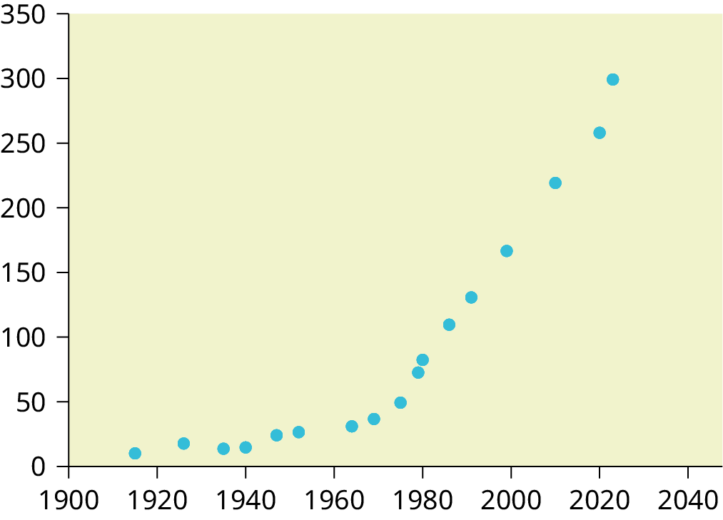
x軸を年、y軸を消費者物価指数としたデータの散布図と最適直線。 — Figure 12.29図 12.29

NOTE注

In the example, notice the pattern of the points compared to the line. Although the correlation coefficient is significant, the pattern in the scatterplot indicates that a curve would be a more appropriate model to use than a line. In this example, a statistician should prefer to use other methods to fit a curve to this data, rather than model the data with the line we found. In addition to doing the calculations, it is always important to look at the scatterplot when deciding whether a linear model is appropriate.

英語のヒント

この例では、直線に対する点の並び方に注目しよう。相関係数は有意だが、散布図の形を見ると、直線より曲線のほうがモデルとして適切だとわかる。この場合、統計学者は、求めた直線でデータをモデル化するよりも、別の方法で曲線を当てはめることを選ぶべきである。線形モデルが適切かどうかを判断するときには、計算を行うだけでなく、散布図を見ることが常に重要である。

If you are interested in seeing more years of data, visit the Bureau of Labor Statistics CPI website ftp://ftp.bls.gov/pub/special.requests/cpi/cpiai.txt; our data is taken from the column entitled "Annual Avg." (third column from the right). For example you could add more current years of data. Try adding the more recent years: 2010: CPI = 219.2; 2020: CPI = 258.0; 2023: CPI = 299.2. See how it affects the model. (Check:

\overset{⏜}{y} = - 5030 + 2.598 x

;

r = 0.9067

. Is r significant? Is the fit better with the addition of the new points?)

英語のヒント

さらに多くの年のデータを見たければ、労働統計局のCPIのウェブサイト ftp://ftp.bls.gov/pub/special.requests/cpi/cpiai.txt を参照しよう。ここで使ったデータは「Annual Avg.」（年平均）という列（右から3列目）から取ったものである。たとえば、より新しい年のデータを追加できる。2010年：CPI = 219.2、2020年：CPI = 258.0、2023年：CPI = 299.2 を追加して、モデルがどう変わるか調べよう。（確認：

\overset{⏜}{y} = - 5030 + 2.598 x

、

r = 0.9067

。r は有意か。新しい点を追加すると当てはまりはよくなるか。）

Try Itやってみよう

The following table shows economic development measured in per capita income PCINC.

英語のヒント

次の表は、1人当たり所得 PCINC で測った経済発展を示している。

Table 12.22表 12.22
Year 年	PCINC	Year 年	PCINC
1870	340	1920	1050
1880	499	1930	1170
1890	592	1940	1364
1900	757	1950	1836
1910	927	1960	2132

What are the independent and dependent variables?
独立変数と従属変数は何か。
Draw a scatter plot.
散布図を描け。
Use regression to find the line of best fit and the correlation coefficient.
回帰を用いて最適直線と相関係数を求めよ。
Interpret the significance of the correlation coefficient.
相関係数の有意性を解釈せよ。
Is there a linear relationship between the variables?
変数間に線形関係はあるか。
Find the coefficient of determination and interpret it.
決定係数を求め、解釈せよ。
What is the slope of the regression equation? What does it mean?
回帰式の傾きはいくつか。それは何を意味するか。
Use the line of best fit to estimate PCINC for 1900, for 2000.
最適直線を用いて、1900年と2000年の PCINC を推定せよ。
Determine if there are any outliers.
外れ値があるかどうかを調べよ。