第12章線形回帰と相関
THIRD-EXAM vs FINAL-EXAM EXAMPLE: critical value method第3回試験と期末試験の例:臨界値法
Consider the third exam/final exam example. The line of best fit is: ŷ = –173.51+4.83x with r = 0.6631 and there are n = 11 data points. Can the regression line be used for prediction? Given a third-exam score (x value), can we use the line to predict the final exam score (predicted y value)?
「第3回試験と期末試験の例」を考えよう。最適な当てはめ直線はŷ = −173.51 + 4.83x、r = 0.6631で、データ点はn = 11個ある。回帰直線を予測に使えるだろうか。第3回試験の得点(x)が与えられたとき、この直線で期末試験の得点(予測値y)を求められるだろうか。
- H0: ρ = 0H0:ρ = 0
- Ha: ρ ≠ 0Ha:ρ ≠ 0
- α = 0.05
- Use the "95% Critical Value" table for r with df = n – 2 = 11 – 2 = 9.df = n − 2 = 11 − 2 = 9として、rの「95%臨界値」表を使う。
- The critical values are –0.602 and +0.602臨界値は−0.602と+0.602である。
- Since 0.6631 > 0.602, r is significant.0.6631 > 0.602なので、rは有意である。
- Decision: Reject the null hypothesis.判断:帰無仮説を棄却する。
- Conclusion:There is sufficient evidence to conclude that there is a significant linear relationship between the third exam score (x) and the final exam score (y) because the correlation coefficient is significantly different from zero.結論:相関係数が0と有意に異なるため、第3回試験の得点xと期末試験の得点yの間に有意な線形関係があると結論する十分な証拠がある。
Because r is significant and the scatter plot shows a linear trend, the regression line can be used to predict final exam scores.
rが有意で散布図も直線的な傾向を示すため、回帰直線を使って期末試験の得点を予測できる。
Example 12.10例題 12.10
Suppose you computed the following correlation coefficients. Using the table at the end of the chapter, determine if r is significant and the line of best fit associated with each r can be used to predict a y value. If it helps, draw a number line.
次の相関係数が得られたとする。章末の表を使い、rが有意で、それぞれに対応する最適直線をyの予測に使えるかを判断しよう。必要なら数直線を描こう。
- r = –0.567 and the sample size, n, is 19. The df = n – 2 = 17. The critical value is –0.456. –0.567 < –0.456 so r is significant.r = −0.567、標本の大きさn = 19。df = n − 2 = 17。臨界値は−0.456。−0.567 < −0.456なので、rは有意である。
- r = 0.708 and the sample size, n, is nine. The df = n – 2 = 7. The critical value is 0.666. 0.708 > 0.666 so r is significant.r = 0.708、標本の大きさn = 9。df = n − 2 = 7。臨界値は0.666。0.708 > 0.666なので、rは有意である。
- r = 0.134 and the sample size, n, is 14. The df = 14 – 2 = 12. The critical value is 0.532. 0.134 is between –0.532 and 0.532 so r is not significant.r = 0.134、標本の大きさn = 14。df = 14 − 2 = 12。臨界値は0.532。0.134は−0.532と0.532の間なので、rは有意ではない。
- r = 0 and the sample size, n, is five. No matter what the dfs are, r = 0 is between the two critical values so r is not significant.r = 0、標本の大きさn = 5。自由度がいくつでも、r = 0は二つの臨界値の間にあるため有意ではない。
Assumptions in Testing the Significance of the Correlation Coefficient相関係数の有意性検定の仮定
Testing the significance of the correlation coefficient requires that certain assumptions about the data are satisfied. The premise of this test is that the data are a sample of observed points taken from a larger population. We have not examined the entire population because it is not possible or feasible to do so. We are examining the sample to draw a conclusion about whether the linear relationship that we see between x and y in the sample data provides strong enough evidence so that we can conclude that there is a linear relationship between x and y in the population.
英語のヒント
相関係数の有意性を検定するには、データについて一定の仮定が満たされている必要がある。この検定は、データがより大きな母集団から得られた観測点の標本であることを前提とする。母集団全体を調べていないのは、それが不可能か、実行可能でないからである。標本データのxとyに見られる線形関係が、母集団でもxとyに線形関係があると結論するのに十分強い証拠となるかを判断するため、標本を調べている。
The regression line equation that we calculate from the sample data gives the best-fit line for our particular sample. We want to use this best-fit line for the sample as an estimate of the best-fit line for the population. Examining the scatterplot and testing the significance of the correlation coefficient helps us determine if it is appropriate to do this.
標本データから計算した回帰直線の方程式は、その特定の標本に最もよく適合する直線を与える。この標本の最適直線を、母集団の最適直線の推定として使いたい。散布図を調べ、相関係数の有意性を検定することで、それが適切かを判断しやすくなる。
- The relationship between the variables being correlated should be linear. The data points should fall along an approximate straight-line pattern when plotted as (x, y) data points on a scatter plot.相関を調べる変数間の関係は線形であるべきだ。散布図に(x, y)の点を描いたとき、点はおおよそ直線状に並ぶべきである。
- The y values for any particular x value are normally distributed about the line. This implies that there are more y values scattered closer to the line than are scattered farther away. Assumption (1) implies that these normal distributions are centered on the line: the means of these normal distributions of y values lie on the line.どの特定のxについても、yの値は直線の周りに正規分布する。これは、直線から遠く離れたyの値より、近くに散らばる値のほうが多いことを意味する。仮定(1)は、これらの正規分布の中心が直線上にあること、つまり各yの正規分布の平均が直線上にあることを意味する。
- The standard deviations of the population y values about the line are equal for each value of x. In other words, each of these normal distributions of y values has the same shape and spread about the line.母集団のyの値の直線の周りでの標準偏差は、xの値によらず等しい。言い換えると、各yの正規分布は、直線の周りで同じ形と広がりを持つ。
- The residual errors are mutually independent (no pattern).
英語のヒント
残差は互いに独立である(パターンがない)。 - The data are produced from a well-designed, random sample or randomized experiment.データは、適切に設計された無作為標本または無作為化実験から得られる。
The assumptions underlying the test of significance are:有意性検定の基礎となる仮定
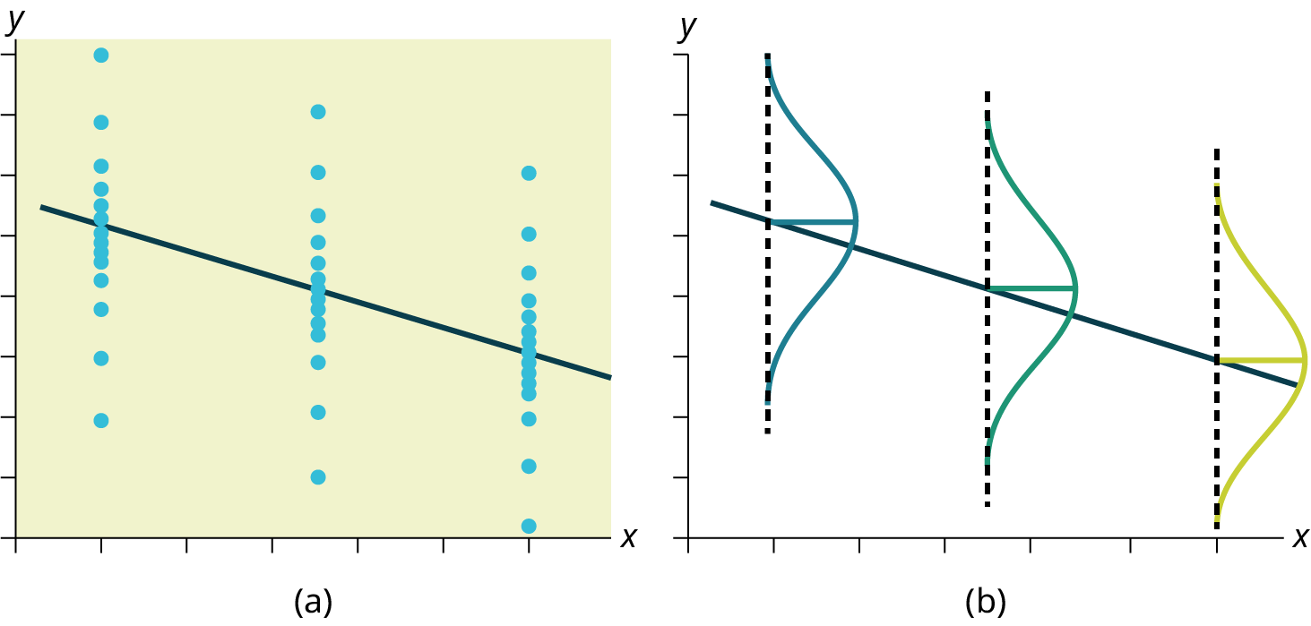

Figure 12.25図 12.25
The y values for each x value are normally distributed about the line with the same standard deviation. For each x value, the mean of the y values lies on the regression line. More y values lie near the line than are scattered further away from the line.
各xのyの値は、直線の周りに同じ標準偏差で正規分布する。各xについて、yの平均は回帰直線上にある。直線から遠くに散らばる値より、近くにあるyの値のほうが多い。