第12章線形回帰と相関
95% Critical Values of the Sample Correlation Coefficient Table標本相関係数の95%臨界値表
Degrees of Freedom: n – 2 自由度:n − 2 |
Critical Values: (+ and –) 臨界値:(+と−) |
|---|---|
1 |
0.997 |
2 |
0.950 |
3 |
0.878 |
4 |
0.811 |
5 |
0.754 |
6 |
0.707 |
7 |
0.666 |
8 |
0.632 |
9 |
0.602 |
10 |
0.576 |
11 |
0.555 |
12 |
0.532 |
13 |
0.514 |
14 |
0.497 |
15 |
0.482 |
16 |
0.468 |
17 |
0.456 |
18 |
0.444 |
19 |
0.433 |
20 |
0.423 |
21 |
0.413 |
22 |
0.404 |
23 |
0.396 |
24 |
0.388 |
25 |
0.381 |
26 |
0.374 |
27 |
0.367 |
28 |
0.361 |
29 |
0.355 |
30 |
0.349 |
40 |
0.304 |
50 |
0.273 |
60 |
0.250 |
70 |
0.232 |
80 |
0.217 |
90 |
0.205 |
100 |
0.195 |
References参考文献
Data from the House Ways and Means Committee, the Health and Human Services Department.
データの出典:下院歳入委員会、保健福祉省。
Data from Microsoft Bookshelf.
データの出典:Microsoft Bookshelf。
Data from the United States Department of Labor, the Bureau of Labor Statistics.
データの出典:米国労働省、労働統計局。
Data from the Physician’s Handbook, 1990.
データの出典:『Physician’s Handbook』、1990年。
Data from the United States Department of Labor, the Bureau of Labor Statistics.
データの出典:米国労働省、労働統計局。
Chapter Review章の復習
To determine if a point is an outlier, do one of the following:
英語のヒント
ある点が外れ値かどうかを判断するには、次のいずれかを行う。
- Input the following equations into the TI 83, 83+,84, 84+:次の式を TI 83、83+、84、84+ に入力する。where s is the standard deviation of the residualsここで、s は残差の標準偏差である。If any point is above y2 or below y3 then the point is considered to be an outlier.y2 より上、または y3 より下にある点は、外れ値とみなす。
- Use the residuals and compare their absolute values to 2s where s is the standard deviation of the residuals. If the absolute value of any residual is greater than or equal to 2s, then the corresponding point is an outlier.残差を使い、その絶対値を 2s と比較する。ここで s は残差の標準偏差である。残差の絶対値が 2s 以上なら、対応する点は外れ値である。
- Note: The calculator function LinRegTTest (STATS TESTS LinRegTTest) calculates s.注:電卓の LinRegTTest 機能(STATS → TESTS → LinRegTTest)で s を計算できる。
Exercises 66–71練習問題 66–71
Use the following information to answer the next four exercises. The scatter plot shows the relationship between hours spent studying and exam scores. The line shown is the calculated line of best fit. The correlation coefficient is 0.69.
次の情報を用いて、続く4問に答えよ。散布図は学習に費やした時間と試験の得点の関係を示している。図の直線は計算で求めた最適直線である。相関係数は0.69である。
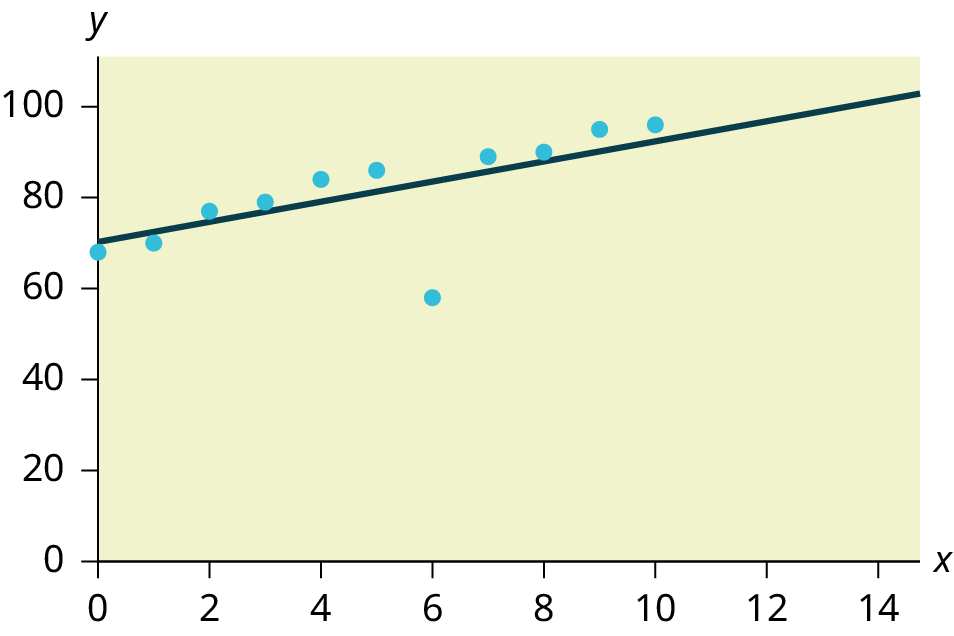

Figure 12.30図 12.30
Exercise 66問題 66
Do there appear to be any outliers?
外れ値があるように見えるか。
Solution解き方
Yes, there appears to be an outlier at (6, 58).
はい、(6, 58) に外れ値があるように見える。
Exercise 67問題 67
A point is removed, and the line of best fit is recalculated. The new correlation coefficient is 0.98. Does the point appear to have been an outlier? Why?
英語のヒント
1点を除いて最適直線を計算し直したところ、新しい相関係数は0.98となった。除いた点は外れ値だったと考えられるか。なぜか。
Exercise 68問題 68
What effect did the potential outlier have on the line of best fit?
外れ値の可能性がある点は、最適直線にどのような影響を与えていたか。
Solution解き方
The potential outlier flattened the slope of the line of best fit because it was below the data set. It made the line of best fit less accurate as a predictor for the data.
英語のヒント
その点はデータの集まりより下にあり、最適直線の傾きを緩くしていた。そのため、データを予測するものとしての最適直線の精度が下がっていた。
Exercise 69問題 69
Are you more or less confident in the predictive ability of the new line of best fit?
英語のヒント
新しい最適直線の予測能力に対する信頼は、以前より高くなるか、低くなるか。
Exercise 70問題 70
The Sum of Squared Errors for a data set of 18 numbers is 49. What is the standard deviation?
18個の数値からなるデータ集合の誤差平方和は49である。標準偏差はいくつか。
Solution解き方
s = 1.75
Exercise 71問題 71
The Standard Deviation for the Sum of Squared Errors for a data set is 9.8. What is the cutoff for the vertical distance that a point can be from the line of best fit to be considered an outlier?
英語のヒント
あるデータ集合の誤差平方和から求めた標準偏差は9.8である。点を外れ値とみなすための、最適直線からの鉛直距離の境界値はいくつか。
Homework宿題
Exercises 72–77練習問題 72–77
Exercise 72問題 72
The height (sidewalk to roof) of notable tall buildings in America is compared to the number of stories of the building (beginning at street level).
英語のヒント
米国の著名な高層ビルについて、高さ(歩道から屋根まで)と階数(地上階から数える)を比較する。
Height (in feet) 高さ(フィート) |
Stories 階数 |
|---|---|
1,050 |
57 |
428 |
28 |
362 |
26 |
529 |
40 |
790 |
60 |
401 |
22 |
380 |
38 |
1,454 |
110 |
1,127 |
100 |
700 |
46 |
- Using “stories” as the independent variable and “height” as the dependent variable, make a scatter plot of the data.「階数」を独立変数、「高さ」を従属変数として、データの散布図を描け。
- Does it appear from inspection that there is a relationship between the variables?図を見て、変数間に関係があるように思えるか。
- Calculate the least squares line. Put the equation in the form of: ŷ = a + bx最小二乗直線を計算し、ŷ = a + bxの形で方程式を書こう。
- Find the correlation coefficient. Is it significant?相関係数を求めよう。有意か。
- Find the estimated heights for 32 stories and for 94 stories.32階建てと94階建てのビルの高さを推定せよ。
- Based on the data in Table 12.24, is there a linear relationship between the number of stories in tall buildings and the height of the buildings?表12.24のデータに基づくと、高層ビルの階数と高さの間に線形関係はあるか。
- Are there any outliers in the data? If so, which point(s)?データに外れ値はあるか。あるなら、どの点か。
- What is the estimated height of a building with six stories? Does the least squares line give an accurate estimate of height? Explain why or why not.6階建てのビルの推定高さはいくつか。最小二乗直線による高さの推定は正確か。その理由を説明せよ。
- Based on the least squares line, adding an extra story is predicted to add about how many feet to a building?最小二乗直線によると、階数が1階増えるごとに、ビルの高さは約何フィート増えると予測されるか。
- What is the slope of the least squares (best-fit) line? Interpret the slope.最小二乗直線(最適直線)の傾きはいくつか。その意味を解釈しよう。
Exercise 73問題 73
Ornithologists, scientists who study birds, tag sparrow hawks in 13 different colonies to study their population. They gather data for the percent of new sparrow hawks in each colony and the percent of those that have returned from migration.
英語のヒント
鳥を研究する科学者である鳥類学者が、ハイタカの個体群を調べるため、13か所のコロニーで個体に標識を付けた。各コロニーで、新たに加わったハイタカの割合と、渡りから戻ってきたハイタカの割合のデータを集めた。
Percent return:74; 66; 81; 52; 73; 62; 52; 45; 62; 46; 60; 46; 38
Percent new:5; 6; 8; 11; 12; 15; 16; 17; 18; 18; 19; 20; 20
Percent new:5; 6; 8; 11; 12; 15; 16; 17; 18; 18; 19; 20; 20
戻ってきた個体の割合:74、66、81、52、73、62、52、45、62、46、60、46、38。新たに加わった個体の割合:5、6、8、11、12、15、16、17、18、18、19、20、20。
- Enter the data into your calculator and make a scatter plot.データを電卓に入力し、散布図を描け。
- Use your calculator’s regression function to find the equation of the least-squares regression line. Add this to your scatter plot from part a.電卓の回帰機能を用いて、最小二乗回帰直線の式を求めよ。それを a の散布図に追加せよ。
- Explain in words what the slope and y-intercept of the regression line tell us.
英語のヒント
回帰直線の傾きと y切片が何を表すかを、言葉で説明せよ。 - How well does the regression line fit the data? Explain your response.回帰直線はデータにどの程度よく当てはまるか。答えの理由を説明せよ。
- Which point has the largest residual? Explain what the residual means in context. Is this point an outlier? An influential point? Explain.残差が最も大きいのはどの点か。その残差がこの状況で何を意味するかを説明せよ。この点は外れ値か。影響の強い点か。説明せよ。
- An ecologist wants to predict how many birds will join another colony of sparrow hawks to which 70% of the adults from the previous year have returned. What is the prediction?
英語のヒント
ある生態学者は、前年の成鳥の70%が戻ってきた別のハイタカのコロニーに、新しい鳥がどれだけ加わるかを予測したい。予測値はいくつか。
Solution解き方
a. and b. Check student’s solution.
a、b。学生の解答を確認する。
c. The slope of the regression line is -0.3031 with a y-intercept of 31.93. In context, the y-intercept indicates that when there are no returning sparrow hawks, there will be almost 32% new sparrow hawks, which doesn’t make sense since if there are no returning birds, then the new percentage would have to be 100% (this is an example of why we do not extrapolate). The slope tells us that for each percentage increase in returning birds, the percentage of new birds in the colony decreases by 30.3%.
c。回帰直線の傾きは −0.3031、y切片は31.93である。この状況で y切片は、戻ってきたハイタカがいないとき、新たに加わったハイタカは約32%になることを示す。しかし、戻ってきた鳥がいなければ新しい鳥の割合は100%でなければならないため、これは意味をなさない(外挿を行わない理由を示す例である)。傾きは、戻ってきた鳥の割合が1%増えるごとに、コロニーに新たに加わった鳥の割合が30.3%減ることを示している。
d. If we examine r2, we see that only 57.52% of the variation in the percent of new birds is explained by the model and the correlation coefficient, r = –.7584 only indicates a somewhat strong correlation between returning and new percentages.
d。r2 を調べると、新しい鳥の割合の変動のうち、モデルで説明できるのは57.52%にすぎない。相関係数 r = −.7584 が示すのも、戻ってきた鳥の割合と新しい鳥の割合の間の、ある程度強い相関にとどまる。
e. The ordered pair (66, 6) generates the largest residual of 6.0. This means that when the observed return percentage is 66%, our observed new percentage, 6%, is almost 6% less than the predicted new value of 11.98%. If we remove this data pair, we see only an adjusted slope of -.2789 and an adjusted intercept of 30.9816. In other words, even though this data generates the largest residual, it is not an outlier, nor is the data pair an influential point.
英語のヒント
e。順序対 (66, 6) が最大の残差6.0を生む。これは、戻ってきた鳥の割合の観測値が66%のとき、新しい鳥の割合の観測値6%が、予測値11.98%より約6%低いことを意味する。このデータ対を除くと、傾きは −.2789、切片は30.9816に変わるだけである。言い換えると、このデータは最大の残差を生むものの、外れ値ではなく、影響の強い点でもない。
f. If there are 70% returning birds, we would expect to see y = –.2789(70) + 30.9816 = 0.114 or 11.4% new birds in the colony.
f。戻ってきた鳥が70%なら、コロニーに新たに加わる鳥は y = −.2789(70) + 30.9816 = 0.114、すなわち11.4%と予想される。
Exercise 74問題 74
The following table shows data on average per capita coffee consumption and heart disease rate in a random sample of 10 countries.
英語のヒント
次の表は、無作為に抽出した10か国における、1人当たりの平均コーヒー消費量と心臓病の割合のデータを示している。
Yearly coffee consumption in liters 年間コーヒー消費量(リットル) |
2.5 |
3.9 |
2.9 |
2.4 |
2.9 |
0.8 |
9.1 |
2.7 |
0.8 |
0.7 |
Death from heart diseases 心臓病による死亡 |
221 |
167 |
131 |
191 |
220 |
297 |
71 |
172 |
211 |
300 |
- Enter the data into your calculator and make a scatter plot.データを電卓に入力し、散布図を描け。
- Use your calculator’s regression function to find the equation of the least-squares regression line. Add this to your scatter plot from part a.電卓の回帰機能を用いて、最小二乗回帰直線の式を求めよ。それを a の散布図に追加せよ。
- Explain in words what the slope and y-intercept of the regression line tell us.回帰直線の傾きと y切片が何を表すかを、言葉で説明せよ。
- How well does the regression line fit the data? Explain your response.回帰直線はデータにどの程度よく当てはまるか。答えの理由を説明せよ。
- Which point has the largest residual? Explain what the residual means in context. Is this point an outlier? An influential point? Explain.残差が最も大きいのはどの点か。その残差がこの状況で何を意味するかを説明せよ。この点は外れ値か。影響の強い点か。説明せよ。
- Do the data provide convincing evidence that there is a linear relationship between the amount of coffee consumed and the heart disease death rate? Carry out an appropriate test at a significance level of 0.05 to help answer this question.
英語のヒント
このデータは、コーヒー消費量と心臓病による死亡率に線形関係があるという説得力のある証拠を示しているか。この問いに答えるため、有意水準0.05で適切な検定を行え。
Exercise 75問題 75
The following table consists of one student athlete’s time (in minutes) to swim 2000 yards and the student’s heart rate (beats per minute) after swimming on a random sample of 10 days:
英語のヒント
次の表は、無作為に選んだ10日間について、ある学生選手が2000ヤードを泳ぐのにかかった時間(分)と、泳いだ後の心拍数(1分当たりの拍動数)を示している。
Swim Time 泳いだ時間 |
Heart Rate 心拍数 |
|---|---|
34.12 |
144 |
35.72 |
152 |
34.72 |
124 |
34.05 |
140 |
34.13 |
152 |
35.73 |
146 |
36.17 |
128 |
35.57 |
136 |
35.37 |
144 |
35.57 |
148 |
- Enter the data into your calculator and make a scatter plot.データを電卓に入力し、散布図を描け。
- Use your calculator’s regression function to find the equation of the least-squares regression line. Add this to your scatter plot from part a.電卓の回帰機能を用いて、最小二乗回帰直線の式を求めよ。それを a の散布図に追加せよ。
- Explain in words what the slope and y-intercept of the regression line tell us.回帰直線の傾きと y切片が何を表すかを、言葉で説明せよ。
- How well does the regression line fit the data? Explain your response.回帰直線はデータにどの程度よく当てはまるか。答えの理由を説明せよ。
- Which point has the largest residual? Explain what the residual means in context. Is this point an outlier? An influential point? Explain.残差が最も大きいのはどの点か。その残差がこの状況で何を意味するかを説明せよ。この点は外れ値か。影響の強い点か。説明せよ。
Solution解き方
- Check student’s solution.学生の解答を確認する。
- Check student’s solution.学生の解答を確認する。
- We have a slope of –1.4946 with a y-intercept of 193.88. The slope, in context, indicates that for each additional minute added to the swim time, the heart rate will decrease by 1.5 beats per minute. If the student is not swimming at all, the y-intercept indicates that his heart rate will be 193.88 beats per minute. While the slope has meaning (the longer it takes to swim 2,000 meters, the less effort the heart puts out), the y-intercept does not make sense. If the athlete is not swimming (resting), then his heart rate should be very low.傾きは −1.4946、y切片は193.88である。この状況で傾きは、泳ぐ時間が1分長くなるごとに、心拍数が1分当たり1.5回減ることを示す。y切片は、学生がまったく泳いでいないときの心拍数が1分当たり193.88回になることを示す。傾きには意味がある(2000メートルを泳ぐのに時間をかけるほど、心臓の負担は小さくなる)が、y切片は意味をなさない。泳いでいないとき(安静時)の心拍数は、かなり低いはずである。
- Since only 1.5% of the heart rate variation is explained by this regression equation, we must conclude that this association is not explained with a linear relationship.この回帰式で説明されるのは心拍数の変動の1.5%にすぎないため、この関連は線形関係では説明できないと結論せざるを得ない。
- The point (34.72, 124) generates the largest residual of –11.82. This means that our observed heart rate is almost 12 beats less than our predicted rate of 136 beats per minute. When this point is removed, the slope becomes –2.953 with the y-intercept changing to 247.1616. While the linear association is still very weak, we see that the removed data pair can be considered an influential point in the sense that the y-intercept becomes more meaningful.
英語のヒント
点 (34.72, 124) が、最大の残差 −11.82 を生む。これは、心拍数の観測値が、予測値である1分当たり136回より約12回少ないことを意味する。この点を除くと、傾きは −2.953、y切片は247.1616になる。線形の関連は依然として非常に弱いが、y切片がより意味のあるものになるという点で、除いたデータ対は影響の強い点と考えられる。
Exercise 76問題 76
A researcher is investigating whether population impacts homicide rate. He uses demographic data from Detroit, MI to compare homicide rates and the number of the population that are White men.
英語のヒント
ある研究者は、人口が殺人発生率に影響するかどうかを調べている。ミシガン州デトロイトの人口統計データを用いて、殺人発生率と白人男性の人口を比較する。
Population Size 人口 |
Homicide rate per 100,000 people 人口10万人当たりの殺人発生率 |
|---|---|
558,724 |
8.6 |
538,584 |
8.9 |
519,171 |
8.52 |
500,457 |
8.89 |
482,418 |
13.07 |
465,029 |
14.57 |
448,267 |
21.36 |
432,109 |
28.03 |
416,533 |
31.49 |
401,518 |
37.39 |
387,046 |
46.26 |
373,095 |
47.24 |
359,647 |
52.33 |
- Use your calculator to construct a scatter plot of the data. What should the independent variable be? Why?電卓を使ってデータの散布図を描け。独立変数は何にすべきか。なぜか。
- Use your calculator’s regression function to find the equation of the least-squares regression line. Add this to your scatter plot.電卓の回帰機能を使って、最小二乗回帰直線の式を求めよ。それを散布図に追加せよ。
- Discuss what the following mean in context.次の値がこの状況で何を意味するかを論じよ。
- The slope of the regression equation回帰式の傾き
- The y-intercept of the regression equation回帰式の y切片
- The correlation r相関係数 r
- The coefficient of determination r2.決定係数 r2。
- Do the data provide convincing evidence that there is a linear relationship between population size and homicide rate? Carry out an appropriate test at a significance level of 0.05 to help answer this question.このデータは、人口と殺人発生率に線形関係があるという説得力のある証拠を示しているか。この問いに答えるため、有意水準0.05で適切な検定を行え。
Exercise 77問題 77
School 大学 |
Mid-Career Salary (in thousands) 中堅期の給与(千ドル) |
Yearly Tuition 年間授業料 |
|---|---|---|
Princeton プリンストン |
137 |
57,410 |
Harvey Mudd ハーヴィー・マッド |
135 |
62,817 |
CalTech カリフォルニア工科大学 |
127 |
60,864 |
US Naval Academy 米国海軍兵学校 |
122 |
0 |
West Point 米国陸軍士官学校 |
120 |
0 |
MIT |
118 |
57,986 |
Lehigh University リーハイ大学 |
118 |
59,930 |
NYU-Poly ニューヨーク大学ポリテクニック |
117 |
58,168 |
Babson College バブソン大学 |
117 |
56,576 |
Stanford スタンフォード |
114 |
56,169 |
Using the data to determine the linear-regression line equation with the outliers removed. Is there a linear correlation for the data set with outliers removed? Justify your answer.
外れ値を除いたデータを用いて、線形回帰直線の式を求めよ。外れ値を除いたデータ集合には線形相関があるか。答えの根拠を示せ。
Solution解き方
If we remove the two service academies (the tuition is $0.00), we construct a new regression equation of y = 0.002x + 0.309 with a correlation coefficient of 0.533 and a coefficient of determination of 0.284. There is not enough evidence to state that there is a strong linear correlation between tuition costs and future salaries, even when the service academies are removed.
英語のヒント
2校の士官学校(授業料は0.00ドル)を除くと、新しい回帰式は y = 0.002x + 0.309、相関係数は0.533、決定係数は0.284となる。士官学校を除いても、授業料と将来の給与に強い線形相関があると言うには証拠が不十分である。