第12章線形回帰と相関

Residuals Plots残差プロット

A residuals plot can be used to help determine if a set of (x, y) data is linearly correlated. For each data point used to create the correlation line, a residual y - ŷ can be calculated, where y is the observed value of the response variable and ŷ is the value predicted by the correlation line. The difference between these values is called the residual. A residuals plot shows the explanatory variable x on the horizontal axis and the residual for that value on the vertical axis. The residuals plot is often shown together with a scatter plot of the data. While a scatter plot of the data should resemble a straight line, a residuals plot should appear random, with no pattern and no outliers. It should also show constant error variance, meaning the residuals should not consistently increase (or decrease) as the explanatory variable x increases.

英語のヒント

残差プロットは、(x, y)データの集合に線形相関があるかを判断するのに役立つ。相関直線の作成に使った各データ点について、残差y − ŷを計算できる。yは応答変数の観測値、ŷは相関直線による予測値である。この差を残差という。残差プロットでは、横軸に説明変数x、縦軸にその値に対応する残差を示す。データの散布図と一緒に示すことが多い。データの散布図は直線に近い形になるべきだが、残差プロットはパターンや外れ値がなく、無作為に見えるべきである。誤差の分散も一定であるべきだ。つまり、説明変数xが増えるにつれて、残差が一貫して増加したり減少したりしてはならない。

A residuals plot can be created using StatCrunch or a TI calculator. The plot should appear random. A box plot of the residuals is also helpful to verify that there are no outliers in the data. By observing the scatter plot of the data, the residuals plot, and the box plot of residuals, together with the linear correlation coefficient, we can usually determine if it is reasonable to conclude that the data are linearly correlated.

英語のヒント

残差プロットはStatCrunchやTI電卓で作れる。プロットは無作為に見えるべきである。残差の箱ひげ図も、データに外れ値がないことを確かめるのに役立つ。データの散布図、残差プロット、残差の箱ひげ図を、線形相関係数と併せて観察すると、通常、データに線形相関があると結論するのが妥当かどうかを判断できる。

EXAMPLE:例：

A shop owner uses a straight-line regression to estimate the number of ice cream cones that would be sold in a day based on the temperature at noon. The owner has data for a 2-year period and chose nine days at random. A scatter plot of the data is shown, together with a residuals plot.

店主が正午の気温をもとに、1日に売れるコーン入りアイスクリームの数を直線回帰で推定する。2年間のデータから9日を無作為に選んだ。データの散布図と残差プロットを示す。

Table 12.10表 12.10
Table showing the number of ice cream cones sold on nine random days and the temperature at noon on those days.
無作為に選んだ9日間のコーン入りアイスクリーム販売数と、各日の正午の気温を示す表。
Temperature ° F 気温（°F）	Ice cream cones sold コーン入りアイスクリーム販売数
70	105
85	240
65	49
72	147
80	231
61	38
75	193
78	196
68	89

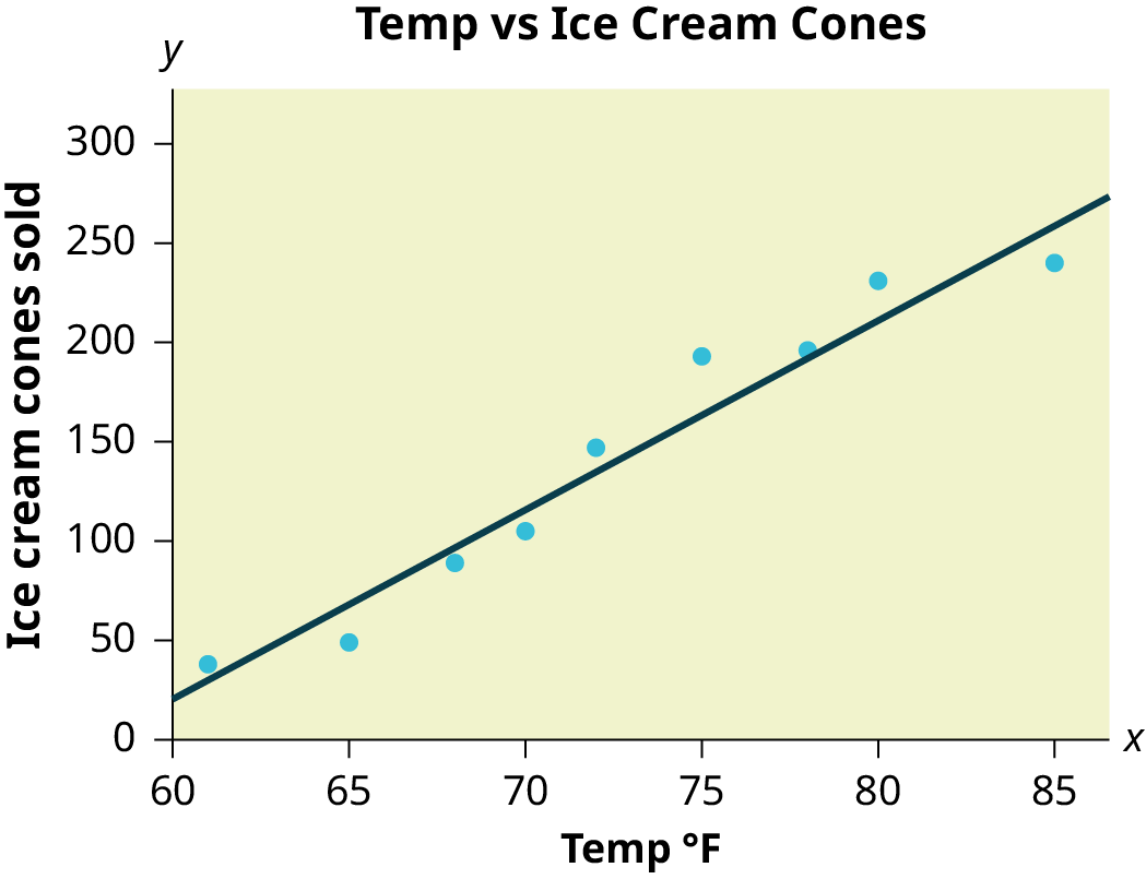
与えられたデータの気温とアイスクリーム販売数の散布図。直線が当てはめられている。 — Figure 12.17図 12.17
Scatter plot of the data looks like a straight line.
データの散布図は、直線のように見える。

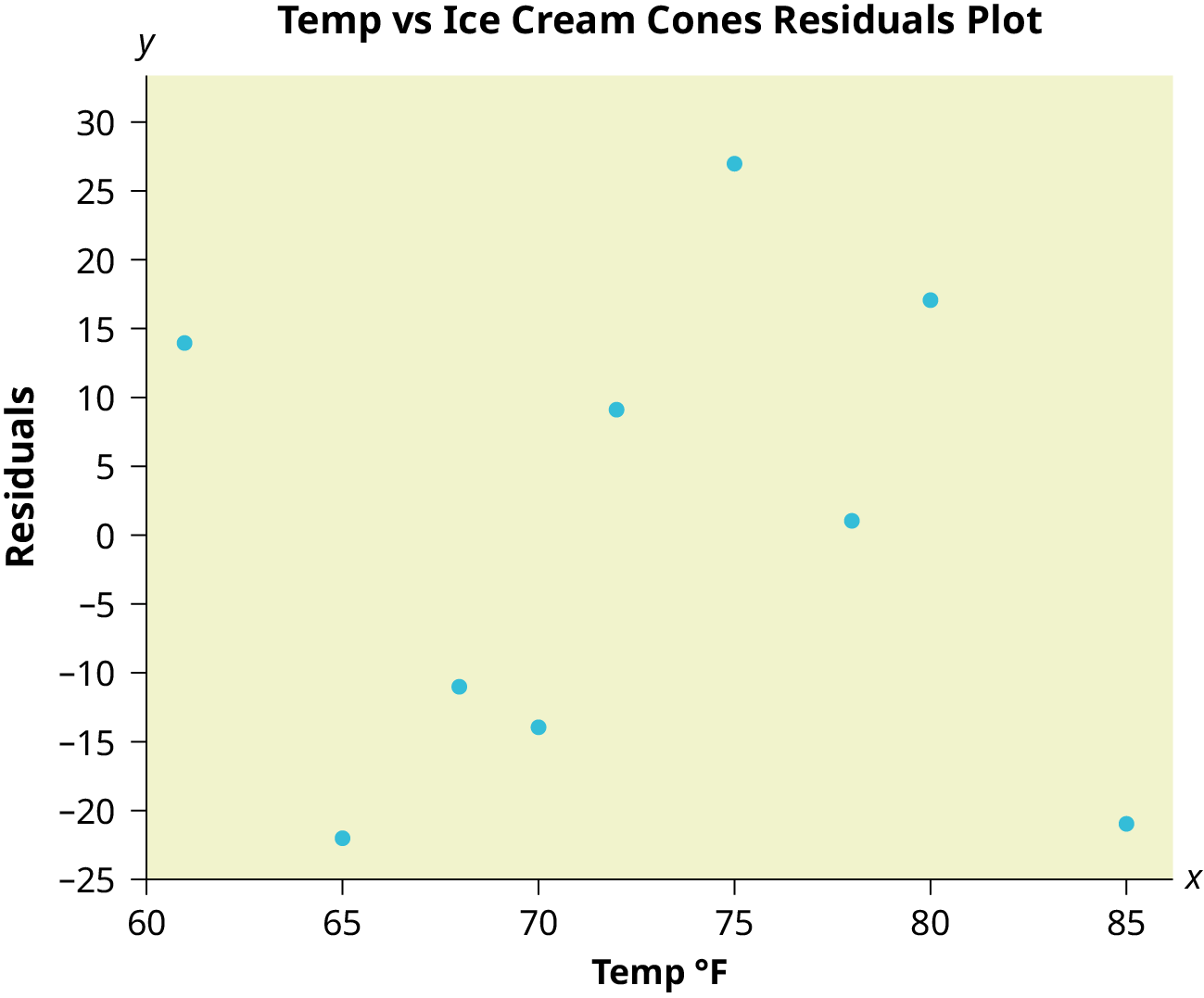
与えられたデータの気温に対する残差を示す残差プロット。 — Figure 12.18図 12.18
Residuals plot appears random.
残差プロットは無作為に見える。

Least Squares Criteria for Best Fit最小二乗法による最適な当てはめの基準

The process of fitting the best-fit line is called linear regression. The idea behind finding the best-fit line is based on the assumption that the data are scattered about a straight line. The criteria for the best fit line is that the sum of the squared errors (SSE) is minimized, that is, made as small as possible. Any other line you might choose would have a higher SSE than the best fit line. This best fit line is called the least-squares regression line .

英語のヒント

最適な直線を当てはめる手順を線形回帰という。その考え方は、データが直線の周りに散らばっているという仮定に基づく。最適な直線の基準は、誤差平方和（SSE）を最小にする、すなわち可能な限り小さくすることである。他のどの直線を選んでも、SSEはこの最適な直線より大きくなる。この直線を最小二乗回帰直線という。

THIRD EXAM vs FINAL EXAM EXAMPLE:第3回試験と期末試験の例：

The graph of the line of best fit for the third-exam/final-exam example is as follows:

第3回試験と期末試験の例で、最適な当てはめ直線のグラフは次のようになる。

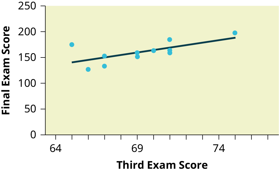
試験得点の散布図と最適な当てはめ直線。一つのデータ点と、それに対応する直線上の点が強調されている。 — Figure 12.19図 12.19

The least squares regression line (best-fit line) for the third-exam/final-exam example has the equation:

第3回試験と期末試験の例で、最小二乗回帰直線（最適な当てはめ直線）の方程式は次のとおりである。

\hat{y} = - 173.51 + 4.83 x

REMINDER確認

Remember, it is always important to plot a scatter diagram first. If the scatter plot indicates that there is a linear relationship between the variables, then it is reasonable to use a best fit line to make predictions for y given x within the domain of x-values in the sample data, but not necessarily for x-values outside that domain. You could use the line to predict the final exam score for a student who earned a grade of 73 on the third exam. You should NOT use the line to predict the final exam score for a student who earned a grade of 50 on the third exam, because 50 is not within the domain of the x-values in the sample data, which are between 65 and 75.

英語のヒント

まず散布図を描くことが常に重要だと覚えておこう。散布図が変数間の線形関係を示す場合、標本データのxの範囲内で与えられたxからyを予測するのに、最適な直線を使うことは妥当である。しかし、その範囲外のxに対しても妥当とは限らない。第3回試験が73点だった学生の期末試験の得点は、この直線で予測できる。第3回試験が50点だった学生の期末試験の得点の予測には、使ってはならない。標本データのxは65～75の範囲であり、50はそこに含まれないからである。