第4章離散確率変数
Notation for the Geometric: G = Geometric Probability Distribution Function幾何分布の表記:G = 幾何確率分布関数
X ~ G(p)
Read this as "X is a random variable with a geometric distribution." The parameter is p; p = the probability of a success for each trial.
これを「Xは幾何分布に従う確率変数である」と読む。母数はpで、p = 各試行で成功する確率である。
CASE I: Random Variable X Is Event of First Success
場合I:確率変数Xが最初の成功の起こる回を表す
In this case we ask, “What is the probability that we will have some number x of events of interest to us of failures before a success?”
この場合、「成功する前に、関心のある失敗という事象がx回起こる確率はいくらか」と問う。
The geometric pdf tells us the probability that the first occurrence of success requires x number of failure independent trials, each with probability . If the probability of success on each trial is p, then the probability that the xth trial (out of x trials) is the first success is:
幾何pdfは、最初に成功するまでに、それぞれ確率の独立な失敗試行がx回必要となる確率を示す。各試行の成功確率がpなら、x回の試行のうちx回目が最初の成功となる確率は、
for
の場合
Like the binomial distribution, the geometric distribution has the parameters of the mean and standard deviation. The expected value of X, the mean for Case I, is This tells us how many failed trials to expect until we get the first success. This count includes in the count of trials the trial that results in success. The above form of the geometric distribution is used for modeling the number of trials until the first success. The number of trials includes the one that is a success: x = all trials including the one that is a success. This can be seen in the form of the formula. If X = number of trials including the success, then we must multiply the probability of failure, , times the number of failures, that is . The standard deviation of Case I of the geometric distribution is:
二項分布と同様、幾何分布にも平均と標準偏差という母数がある。Xの期待値、すなわち場合Iの平均はである。これにより、最初の成功までに何回の失敗が予想されるかが分かる。この試行回数には、成功する試行も含まれる。上の形の幾何分布は、最初の成功までの試行回数をモデル化する。成功した1回も含むので、x = 成功した回を含めた全試行回数となる。これは公式の形からも分かる。X = 成功した回を含む試行回数なら、失敗確率を失敗回数、すなわち回掛け合わせる必要がある。場合Iの幾何分布の標準偏差は、
CASE II: Random Variable X Is Number of Failures BEFORE a Success
場合II:確率変数Xが成功前の失敗回数を表す
By contrast to Case I, the following form of the geometric distribution used for modeling number of failures until the first success is:
場合Iと対照的に、最初の成功までの失敗回数をモデル化する幾何分布は、次の形をとる。
for
の場合
In this case the trial that is the success is not counted as a trial in the formula: x = number of failures. The expected value, the mean, of this distribution is . This tells us how many failures to expect before we have a success. In either case, the sequence of probabilities is a geometric sequence. In Case II, the standard deviation parameter is:
この場合、成功した試行は公式中の試行回数に数えず、x = 失敗回数とする。この分布の期待値、すなわち平均はである。これにより、成功する前に何回失敗すると予想されるかが分かる。どちらの場合も、確率の列は等比数列である。場合IIの標準偏差の母数はである。
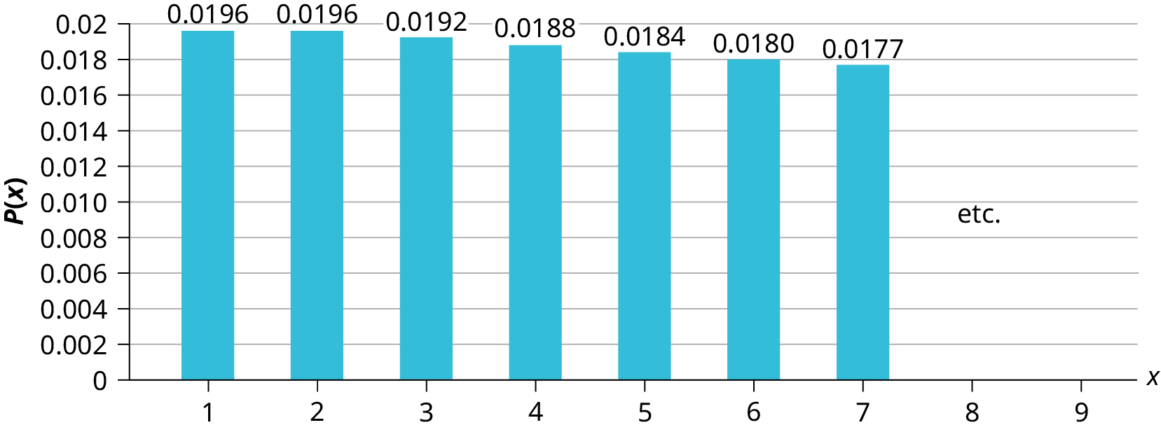

Figure 4.5図 4.5
The y-axis in Figure 4.5 contains the probability of x, and the x-axis is the random number components tested. For example, at the probability it will be found to be defective is 0.0196. With two components tested, the probability the second component is defective is graphed at a probability of 0.0196 at on the x axis. For the probability that the third component is defective we find (The first two are the same because of rounding in the computations.)
図4.5のy軸はxの確率を表し、x軸は検査した部品の個数という確率変数を表す。たとえば、で不良品が見つかる確率は0.0196である。2個検査するとき、2個目が不良品である確率は、x軸のの位置に0.0196として描かれる。3個目が不良品である確率はとなる(最初の二つが同じなのは、計算時に丸めているためである)。
Notice on Figure 4.5 that the probabilities decline by the same step down with each change in the value of x. This increment is called the common ratio. This exists for the geometric probability distribution uniquely. The common ratio, called r, can be calculated by dividing any value by the previous value, e.g.,
英語のヒント
図4.5では、xの値が変わるたびに確率が同じ段階で減少することに注意しよう。この変化を公比と呼ぶ。これは幾何確率分布特有の性質である。rと呼ばれる公比は、任意の値をその直前の値で割ることで求められる。たとえば、
For this set of data, therefore, the common ratio is 0.98. The common ratio then multiplied by any other probability value will provide the next probability value in the sequence. For example, the probability that the sixth component tested is a failure is 0.018078. Check this using the formula from Case I. Now we have the . Knowing this and the common ratio we can calculate the by simple multiplication: , the same value we found earlier by using the geometric probability distribution. This common ratio increment is the same ratio between every number and is called a geometric progression and thus the name for this probability density function. Once the common ratio is calculated, any one desires to know can be easily found.
英語のヒント
したがって、このデータの公比は0.98である。ほかのどの確率の値に公比を掛けても、数列の次の確率が得られる。たとえば、検査した6個目が不良品である確率は0.018078である。場合Iの公式を使って確認せよ。これでが分かった。この値と公比から、単純な掛け算でを計算できる。となり、先に幾何確率分布で求めた値と一致する。各数の間で同じ比率で変化するこの並びは等比数列と呼ばれ、この確率密度関数の名称の由来でもある。公比が分かれば、知りたいどのも簡単に求められる。
The number of components that you would expect to test until you find the first defective component is the mean, for this case of defective components. The formula for the mean of the geometric distribution for the random variable defined as number of failures before first success is
最初の不良部品が見つかるまでに検査すると予想される部品数は平均であり、この不良部品の例ではである。最初の成功前の失敗回数として定義した確率変数について、幾何分布の平均の公式はとなる。
See Example 4.20 for an example where the geometric random variable is defined as number of trials until first success. The expected value of this formula for the geometric distribution will be different from this version of the distribution. Case II also has a variance, but this is changed from the Case I formula. This formula for the variance is:
幾何確率変数を最初の成功までの試行回数として定義した例は、例4.20を参照せよ。この幾何分布の公式による期待値は、こちらの形の分布とは異なる。場合IIにも分散があるが、その公式は場合Iから変わる。分散の公式は次のとおりである。
for
の場合
The formula for the variance is分散の公式は、
The standard deviation is標準偏差は、
Example 4.20例題 4.20
Assume that the probability of a defective computer component is 0.02. Components are randomly selected. Find the probability that the first defect is caused by the seventh component tested. How many components do you expect to test until one is found to be defective?
英語のヒント
コンピューター部品が不良品である確率を0.02とする。部品は無作為に選ばれる。検査した7個目が最初の不良部品となる確率を求めよ。不良品が一つ見つかるまでに、何個検査すると予想されるか。
Let X = the number of computer components tested until the first defect is found.
X = 最初の不良品が見つかるまでに検査するコンピューター部品の個数とする。
X takes on the values 1, 2, 3, ... where p = 0.02.
Xは1、2、3、…の値を取り、p = 0.02である。
Find P(x = 7). P(x = 7) = 0.0177.
P(x = 7)を求める。P(x = 7) = 0.0177である。
Using the Calculator電卓の操作
To find the probability that x ≤ 7, follow the same instructions EXCEPT select E:geometcdf(as the distribution function.
x ≤ 7となる確率を求めるには、分布関数としてE:geometcdf(を選ぶ点だけを変え、同じ手順に従う。
The probability that the seventh component is the first defect is 0.0177.
7個目の部品が最初の不良品となる確率は0.0177である。
The formula for the variance is σ2 = = = 2,450
分散の公式は、σ2 = = = 2,450である。
The standard deviation is σ = = = 49.5
標準偏差は、σ = = = 49.5である。
Example 4.21例題 4.21
The lifetime risk of developing cancer is about one in 67 (1.5%). Let X = the number of people you ask until one says they have cancer. Then X is a discrete random variable with a geometric distribution: or
生涯にがんを発症するリスクは約67人に1人(1.5%)である。X = がんにかかっていると答える人が1人見つかるまでに尋ねる人数とする。このとき、Xは幾何分布に従う離散確率変数で、またはと表される。
- What is the probability of that you ask ten people before one says they have cancer?がんにかかっていると答える人が1人見つかるまでに、10人に尋ねる確率はいくらか。
- What is the probability that you must ask 20 people?20人に尋ねる必要がある確率はいくらか。
- Find the (i) mean and (ii) standard deviation of X.Xの(i)平均と(ii)標準偏差を求めよ。
Solution解き方