第5章積分

Exercises 246–248練習問題 246–248

For the next two exercises use the data in the following table, which displays bald eagle populations from 1963 to 2000 in the continental United States.

次の2問では、1963年から2000年までの米国本土におけるハクトウワシの個体群を示した表を使う。

Population of Breeding Bald Eagle Pairsハクトウワシの繁殖つがい数

Table 5.10表 5.10
*Source*: http://www.fws.gov/Midwest/eagle/population/chtofprs.html.
出典：http://www.fws.gov/Midwest/eagle/population/chtofprs.html。
Year 年	Population of Breeding Pairs of Bald Eagles 繁殖中のハクトウワシのつがい数
1963	487
1974	791
1981	1188
1986	1875
1992	3749
1996	5094
2000	6471

Exercise 246問題 246

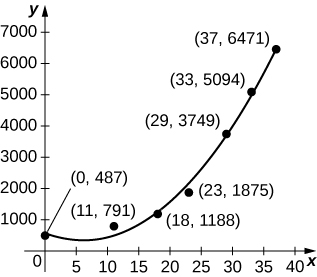
[T] The graph below plots the quadratic

p (t) = 6.48 t^{2} - 80.3 1 t + 585.69

against the data in preceding table, normalized so that

t = 0

corresponds to 1963. Estimate the average number of bald eagles per year present for the 37 years by computing the average value of p over

[0, 37] .

英語のヒント

[T] 次の図は、1963年を

t = 0

として、前の表のデータと二次関数

p (t) = 6.48 t^{2} - 80.3 1 t + 585.69

を重ねたものである。区間

[0, 37]

での p の平均値を計算し、この37年間の年間平均つがい数を見積もれ。

OpenStax, Rice University; Calculus Volume 1. · CC BY-NC-SA 4.0

Exercise 247問題 247

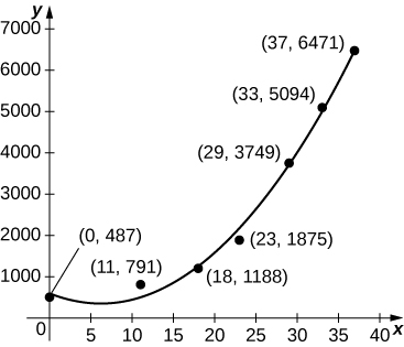
[T] The graph below plots the cubic

p (t) = 0.07 t^{3} + 2.42 t^{2} - 25.63 t + 521.23

against the data in the preceding table, normalized so that

t = 0

corresponds to 1963. Estimate the average number of bald eagles per year present for the 37 years by computing the average value of p over

[0, 37] .

[T] 次の図は、1963年を

t = 0

として、前の表のデータと三次関数

p (t) = 0.07 t^{3} + 2.42 t^{2} - 25.63 t + 521.23

を重ねたものである。区間

[0, 37]

での p の平均値を計算し、この37年間の年間平均つがい数を見積もれ。

OpenStax, Rice University; Calculus Volume 1. · CC BY-NC-SA 4.0

Solution解き方

\frac{1}{37} \int_{0}^{37} p (t) d t = \frac{0.07 {(37)}^{3}}{4} + \frac{2.42 {(37)}^{2}}{3} - \frac{25.63 (37)}{2} + 521.23 \approx 2037

\frac{1}{37} \int_{0}^{37} p (t) d t = \frac{0.07 {(37)}^{3}}{4} + \frac{2.42 {(37)}^{2}}{3} - \frac{25.63 (37)}{2} + 521.23 \approx 2037

Exercise 248問題 248

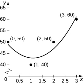
[T] Suppose you go on a road trip and record your speed at every half hour, as compiled in the following table. The best quadratic fit to the data is

q (t) = 5 t^{2} - 11 t + 49,

shown in the accompanying graph. Integrate q to estimate the total distance driven over the 3 hours.

[T] ドライブ中の速さを30分ごとに記録したところ、次の表のようになった。データに最もよく当てはまる二次関数は

q (t) = 5 t^{2} - 11 t + 49,

であり、図に示してある。q を積分して、3時間の総走行距離を見積もれ。

Time (hr) 時間（時間）	Speed (mph) 速さ（mph）
0 (start) 0（出発）	50
1	40
2	50
3	60

OpenStax, Rice University; Calculus Volume 1. · CC BY-NC-SA 4.0

Exercises 249–253練習問題 249–253

As a car accelerates, it does not accelerate at a constant rate; rather, the acceleration is variable. For the following exercises, use the following table, which contains the acceleration measured at every second as a driver merges onto a freeway.

車の加速では、加速度は一定とは限らず変化する。次の各問では、運転者が高速道路に合流する際の加速度を毎秒記録した表を使う。

Time (sec) 時間（秒）	Acceleration (mph/sec) 加速度（mph／秒）
1	11.2
2	10.6
3	8.1
4	5.4
5	0

Exercise 249問題 249

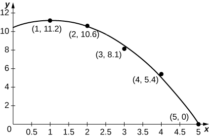
[T] The accompanying graph plots the best quadratic fit,

a (t) = −0.70 t^{2} + 1.44 t + 10.44,

to the data from the preceding table. Compute the average value of

a (t)

to estimate the average acceleration between

t = 0

and

t = 5 .

[T] 図は、前の表のデータに最もよく当てはまる二次関数

a (t) = −0.70 t^{2} + 1.44 t + 10.44

を示している。

a (t)

の平均値を求め、

t = 0

から

t = 5

までの平均加速度を見積もれ。

OpenStax, Rice University; Calculus Volume 1. · CC BY-NC-SA 4.0

Solution解き方

Average acceleration is

A = \frac{1}{5} \int_{0}^{5} a (t) d t = - \frac{0.7 (5^{2})}{3} + \frac{1.44 (5)}{2} + 10.44 \approx 8.2

mph/s

平均加速度は

A = \frac{1}{5} \int_{0}^{5} a (t) d t = - \frac{0.7 (5^{2})}{3} + \frac{1.44 (5)}{2} + 10.44 \approx 8.2

mph/sである。

Exercise 250問題 250

[T] Using your acceleration equation from the previous exercise, find the corresponding velocity equation. Assuming the initial velocity is 0 mph, find the velocity at time

t = 0 .

[T] 前問の加速度の式を使い、対応する速度の式を求めよ。初速を0 mphとすると、時刻

t = 0

の速度はいくらか。

Exercise 251問題 251

[T] Using your velocity equation from the previous exercise, find the corresponding distance equation, assuming your initial distance is 0 mi. How far did you travel while you accelerated your car? (Hint: You will need to convert time units.)

[T] 前問の速度の式を使い、初期位置を0マイルとして、対応する距離の式を求めよ。加速中にどれだけ進んだか。（ヒント：時間の単位を換算する必要がある。）

Solution解き方

d = \int_{0}^{5} |v (t) d t| = \int_{0}^{5} (- \frac{7}{30} t^{3} + 0.72 t^{2} - 10.44 t) d t = 124.042 (\frac{5280}{3600}) = 181.928 ft .

d = \int_{0}^{5} |v (t) d t| = \int_{0}^{5} (- \frac{7}{30} t^{3} + 0.72 t^{2} - 10.44 t) d t = 124.042 (\frac{5280}{3600}) = 181.928 ft

Exercise 252問題 252

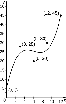
[T] The number of hamburgers sold at a restaurant throughout the day is given in the following table, with the accompanying graph plotting the best cubic fit to the data,

b (t) = 0.12 t^{3} - 2.13 t^{2} + 12.13 t + 3.91,

with

t = 0

corresponding to 9 a.m. and

t = 12

corresponding to 9 p.m. Compute the average value of

b (t)

to estimate the average number of hamburgers sold per hour.

[T] あるレストランで1日の各時間帯に売れたハンバーガー数を表に示す。図は、データに最もよく当てはまる三次関数

b (t) = 0.12 t^{3} - 2.13 t^{2} + 12.13 t + 3.91

を示しており、

t = 0

は午前9時、

t = 12

は午後9時に対応する。

b (t)

の平均値を計算し、1時間当たりの平均販売数を見積もれ。

Hours Past Midnight 午前0時からの経過時間	No. of Burgers Sold ハンバーガー販売数
9	3
12	28
15	20
18	30
21	45

OpenStax, Rice University; Calculus Volume 1. · CC BY-NC-SA 4.0

Exercise 253問題 253

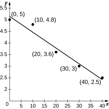
[T] An athlete runs by a motion detector, which records her speed, as displayed in the following table. The best linear fit to this data,

ℓ (t) = −0.068 t + 5.14,

is shown in the accompanying graph. Use the average value of

ℓ (t)

between

t = 0

and

t = 40

to estimate the runner’s average speed.

[T] 運動検出器で記録した選手の速さを表に示す。図は、データに最もよく当てはまる一次関数

ℓ (t) = −0.068 t + 5.14,

を示す。

t = 0

から

t = 40

までの

ℓ (t)

の平均値を使い、選手の平均の速さを見積もれ。

Minutes 分	Speed (m/sec) 速さ（m/s）
0	5
10	4.8
20	3.6
30	3.0
40	2.5

OpenStax, Rice University; Calculus Volume 1. · CC BY-NC-SA 4.0

Solution解き方

\frac{1}{40} \int_{0}^{40} (−0.068 t + 5.14) d t = - \frac{0.068 (40)}{2} + 5.14 = 3.78 m/sec

\frac{1}{40} \int_{0}^{40} (−0.068 t + 5.14) d t = - \frac{0.068 (40)}{2} + 5.14 = 3.78 m/sec

net change theorem

正味の変化の定理

if we know the rate of change of a quantity, the net change theorem says the future quantity is equal to the initial quantity plus the integral of the rate of change of the quantity

ある量の変化率がわかっていれば、変化後の量は、初期値に変化率の積分を加えたものに等しいと述べる定理。