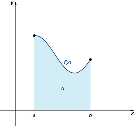
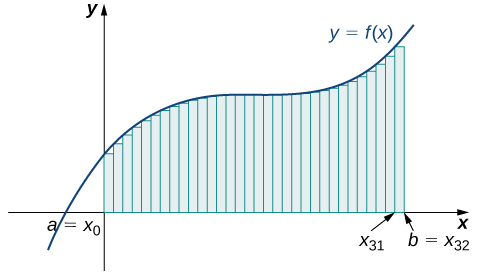
Now that we have the necessary notation, we return to the problem at hand: approximating the area under a curve. Let be a continuous, nonnegative function defined on the closed interval We want to approximate the area A bounded by above, the x-axis below, the line on the left, and the line on the right (Figure 5.2).
英語のヒント
必要な記法がそろったので、曲線の下の面積を近似するという本題に戻ろう。 を、閉区間 で定義された連続かつ非負の関数とする。上を 、下を x 軸、左を直線 、右を直線 で囲まれた領域の面積 A を近似したい(図5.2)。
OpenStax, Rice University; Calculus Volume 1. · CC BY-NC-SA 4.0
Figure 5.2図 5.2
An area (shaded region) bounded by the curve at top, the x-axis at bottom, the line to the left, and the line at right.
上を曲線 、下を x 軸、左を直線 、右を直線 で囲まれた領域(網掛け部分)。
How do we approximate the area under this curve? The approach is a geometric one. By dividing a region into many small shapes that have known area formulas, we can sum these areas and obtain a reasonable estimate of the true area. We begin by dividing the interval into n subintervals of equal width, We do this by selecting equally spaced points with and
英語のヒント
この曲線の下の面積を、どう近似すればよいだろうか。ここでは幾何学的な方法を使う。領域を、面積の公式がわかっている小さな図形に数多く分け、その面積を足し合わせれば、真の面積に近い値を得られる。まず区間 を、幅が等しい n 個の小区間に分ける。それぞれの幅は である。具体的には、 を満たす等間隔の点 を選び、次のように定める。
for
ただし とする。
We denote the width of each subinterval with the notation Δx, so and
英語のヒント
各小区間の幅を Δx と書く。したがって であり、次のようになる。
for This notion of dividing an interval into subintervals by selecting points from within the interval is used quite often in approximating the area under a curve, so let’s define some relevant terminology.
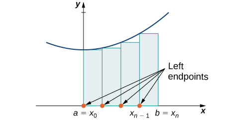
We can use this regular partition as the basis of a method for estimating the area under the curve. We next examine two methods: the left-endpoint approximation and the right-endpoint approximation.
OpenStax, Rice University; Calculus Volume 1. · CC BY-NC-SA 4.0
Figure 5.3図 5.3
In the left-endpoint approximation of area under a curve, the height of each rectangle is determined by the function value at the left of each subinterval.
曲線の下の面積を左端近似するとき、各長方形の高さは各小区間の左端での関数値によって決まる。
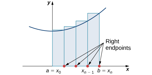
The second method for approximating area under a curve is the right-endpoint approximation. It is almost the same as the left-endpoint approximation, but now the heights of the rectangles are determined by the function values at the right of each subinterval.
OpenStax, Rice University; Calculus Volume 1. · CC BY-NC-SA 4.0
Figure 5.4図 5.4
In the right-endpoint approximation of area under a curve, the height of each rectangle is determined by the function value at the right of each subinterval. Note that the right-endpoint approximation differs from the left-endpoint approximation in Figure 5.3.
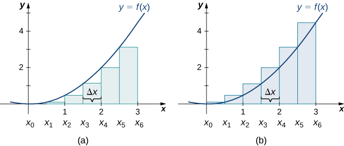
The graphs in Figure 5.5 represent the curve In graph (a) we divide the region represented by the interval into six subintervals, each of width 0.5. Thus, We then form six rectangles by drawing vertical lines perpendicular to the left endpoint of each subinterval. We determine the height of each rectangle by calculating for The intervals are We find the area of each rectangle by multiplying the height by the width. Then, the sum of the rectangular areas approximates the area between and the x-axis. When the left endpoints are used to calculate height, we have a left-endpoint approximation. Thus,
OpenStax, Rice University; Calculus Volume 1. · CC BY-NC-SA 4.0
Figure 5.5図 5.5
Methods of approximating the area under a curve by using (a) the left endpoints and (b) the right endpoints.
曲線の下の面積を、(a)左端、(b)右端を用いて近似する方法。
In Figure 5.5(b), we draw vertical lines perpendicular to such that is the right endpoint of each subinterval, and calculate for We multiply each by Δx to find the rectangular areas, and then add them. This is a right-endpoint approximation of the area under Thus,
Use both left-endpoint and right-endpoint approximations to approximate the area under the curve of on the interval use
区間 で曲線 の下の面積を、左端近似と右端近似の両方を使って近似せよ。 とする。
Solution解き方
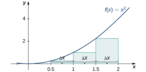
First, divide the interval into n equal subintervals. Using This is the width of each rectangle. The intervals are shown in Figure 5.6. Using a left-endpoint approximation, the heights are Then,
まず区間 を n 個の等しい小区間に分ける。 となり、これが各長方形の幅である。小区間 を図5.6に示す。左端近似では、高さは となる。したがって、
OpenStax, Rice University; Calculus Volume 1. · CC BY-NC-SA 4.0
Figure 5.6図 5.6
The graph shows the left-endpoint approximation of the area under from 0 to 2.
0から2までの の下の面積の左端近似。
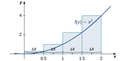
The right-endpoint approximation is shown in Figure 5.7. The intervals are the same, but now use the right endpoint to calculate the height of the rectangles. We have
OpenStax, Rice University; Calculus Volume 1. · CC BY-NC-SA 4.0
Figure 5.7図 5.7
The graph shows the right-endpoint approximation of the area under from 0 to 2.
0から2までの の下の面積の右端近似。
The left-endpoint approximation is 1.75; the right-endpoint approximation is 3.75.
左端近似は1.75、右端近似は3.75となる。
Looking at Figure 5.5 and the graphs in Example 5.4, we can see that when we use a small number of intervals, neither the left-endpoint approximation nor the right-endpoint approximation is a particularly accurate estimate of the area under the curve. However, it seems logical that if we increase the number of points in our partition, our estimate of A will improve. We will have more rectangles, but each rectangle will be thinner, so we will be able to fit the rectangles to the curve more precisely.
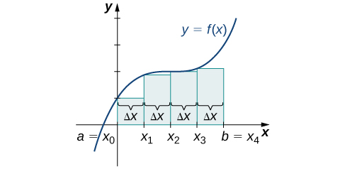
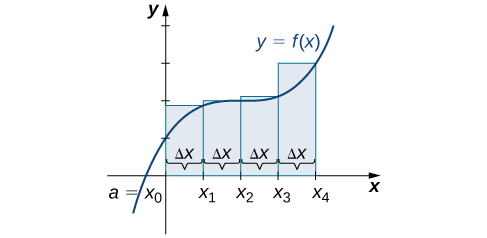
We can demonstrate the improved approximation obtained through smaller intervals with an example. Let’s explore the idea of increasing n, first in a left-endpoint approximation with four rectangles, then eight rectangles, and finally 32 rectangles. Then, let’s do the same thing in a right-endpoint approximation, using the same sets of intervals, of the same curved region. Figure 5.8 shows the area of the region under the curve on the interval using a left-endpoint approximation where The width of each rectangle is
The area is approximated by the summed areas of the rectangles, or
各長方形の面積を足し合わせて、面積を次のように近似する。
OpenStax, Rice University; Calculus Volume 1. · CC BY-NC-SA 4.0
Figure 5.8図 5.8
With a left-endpoint approximation and dividing the region from a to b into four equal intervals, the area under the curve is approximately equal to the sum of the areas of the rectangles.
a から b までを四つの等しい区間に分けて左端近似すると、曲線の下の面積は長方形の面積の和にほぼ等しい。
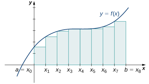
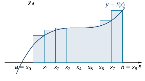
Figure 5.9 shows the same curve divided into eight subintervals. Comparing the graph with four rectangles in Figure 5.8 with this graph with eight rectangles, we can see there appears to be less white space under the curve when This white space is area under the curve we are unable to include using our approximation. The area of the rectangles is
OpenStax, Rice University; Calculus Volume 1. · CC BY-NC-SA 4.0
Figure 5.9図 5.9
The region under the curve is divided into rectangular areas of equal width for a left-endpoint approximation.
左端近似のために、曲線の下の領域を、 として、幅の等しい長方形で近似する。
The graph in Figure 5.10 shows the same function with 32 rectangles inscribed under the curve. There appears to be little white space left. The area occupied by the rectangles is
OpenStax, Rice University; Calculus Volume 1. · CC BY-NC-SA 4.0
Figure 5.10図 5.10
Here, 32 rectangles are inscribed under the curve for a left-endpoint approximation.
左端近似のために、曲線の下に32個の長方形を入れた図。
We can carry out a similar process for the right-endpoint approximation method. A right-endpoint approximation of the same curve, using four rectangles (Figure 5.11), yields an area
OpenStax, Rice University; Calculus Volume 1. · CC BY-NC-SA 4.0
Figure 5.13図 5.13
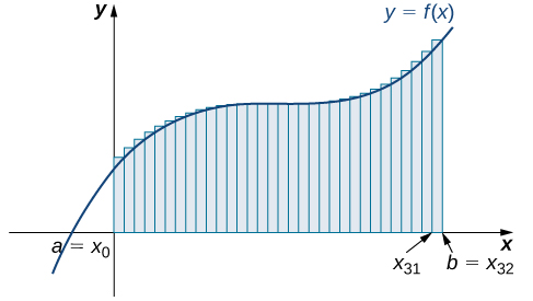
The region is divided into 32 equal subintervals for a right-endpoint approximation.
右端近似のため、領域を32個の等しい小区間に分けた図。
Based on these figures and calculations, it appears we are on the right track; the rectangles appear to approximate the area under the curve better as n gets larger. Furthermore, as n increases, both the left-endpoint and right-endpoint approximations appear to approach an area of 8 square units. Table 5.1 shows a numerical comparison of the left- and right-endpoint methods. The idea that the approximations of the area under the curve get better and better as n gets larger and larger is very important, and we now explore this idea in more detail.