第5章積分
Forming Riemann Sumsリーマン和を作る
So far we have been using rectangles to approximate the area under a curve. The heights of these rectangles have been determined by evaluating the function at either the right or left endpoints of the subinterval In reality, there is no reason to restrict evaluation of the function to one of these two points only. We could evaluate the function at any point in the subinterval and use as the height of our rectangle. This gives us an estimate for the area of the form
英語のヒント
ここまでは、長方形を使って曲線の下の面積を近似してきた。長方形の高さは、小区間 の右端または左端での関数値から決めていた。しかし実際には、関数値を求める点をこの二つだけに限定する必要はない。小区間 内の好きな点 で関数値を求め、 を長方形の高さに使ってもよい。この場合、面積の近似値は次の形になる。
A sum of this form is called a Riemann sum, named for the 19th-century mathematician Bernhard Riemann, who developed the idea.
英語のヒント
この形の和を「リーマン和」という。この考え方を発展させた19世紀の数学者ベルンハルト・リーマンにちなんだ名前である。
Recall that with the left- and right-endpoint approximations, the estimates seem to get better and better as n get larger and larger. The same thing happens with Riemann sums. Riemann sums give better approximations for larger values of n. We are now ready to define the area under a curve in terms of Riemann sums.
英語のヒント
左端近似でも右端近似でも、n を大きくすると近似が次第に正確になるように見えたことを思い出そう。リーマン和でも同じことが起こる。n の値が大きいほど、リーマン和による近似はよくなる。これで、曲線の下の面積をリーマン和によって定義する準備が整った。
Some subtleties here are worth discussing. First, note that taking the limit of a sum is a little different from taking the limit of a function as x goes to infinity. Limits of sums are discussed in detail in the chapter on Sequences and Series; however, for now we can assume that the computational techniques we used to compute limits of functions can also be used to calculate limits of sums.
英語のヒント
ここには、少し注意して考えるべき点がある。まず、和の極限をとることは、x を無限大へ近づけたときの関数 の極限をとることとは少し異なる。和の極限は「数列と級数」の章で詳しく扱う。ここでは、関数の極限の計算に用いた手法を、和の極限の計算にも使えると考えて進めよう。
Second, we must consider what to do if the expression converges to different limits for different choices of Fortunately, this does not happen. Although the proof is beyond the scope of this text, it can be shown that if is continuous on the closed interval then exists and is unique (in other words, it does not depend on the choice of
英語のヒント
次に、 の選び方によって和が異なる極限へ収束するとしたら、どう扱うかを考えなければならない。幸い、この心配は起こらない。証明は本書の範囲を超えるが、 が閉区間 上で連続ならば、 は存在し、しかも一意であることが示せる。言い換えれば、 の選び方には依存しない。
We look at some examples shortly. But, before we do, let’s take a moment and talk about some specific choices for Although any choice for gives us an estimate of the area under the curve, we don’t necessarily know whether that estimate is too high (overestimate) or too low (underestimate). If it is important to know whether our estimate is high or low, we can select our value for to guarantee one result or the other.
英語のヒント
まもなく具体例を見るが、その前に、 の特定の選び方について少し考えよう。 をどのように選んでも曲線の下の面積の近似値は得られるが、その値が真の面積より大きい「過大評価」なのか、小さい「過小評価」なのかは、必ずしもわからない。近似値が大きめか小さめかを知ることが重要な場合は、どちらかになるよう保証する の選び方ができる。
If we want an overestimate, for example, we can choose such that for for all In other words, we choose so that for is the maximum function value on the interval If we select in this way, then the Riemann sum is called an upper sum. Similarly, if we want an underestimate, we can choose so that for is the minimum function value on the interval In this case, the associated Riemann sum is called a lower sum. Note that if is either increasing or decreasing throughout the interval then the maximum and minimum values of the function occur at the endpoints of the subintervals, so the upper and lower sums are just the same as the left- and right-endpoint approximations.
英語のヒント
例えば過大評価がほしければ、すべての に対して が成り立つように を選べばよい。つまり、 に現れる関数値が小区間 上の最大値となるように を選ぶ。このように を選んだリーマン和 を「上和」という。同様に、過小評価がほしければ、 に現れる関数値が小区間 上の最小値となるように を選べばよい。このときのリーマン和を「下和」という。 が区間 全体で増加または減少していれば、各小区間での最大値と最小値は端点でとられる。したがって、この場合の上和・下和は、左端近似・右端近似と一致する。
Example 5.5例題 5.5
Finding Lower and Upper Sums下和と上和を求める
Find a lower sum for on let subintervals.
区間 上の について、 個の小区間を用いて下和を求めよ。
Solution解き方
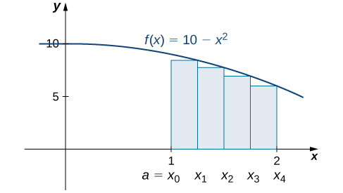
With over the interval We can list the intervals as Because the function is decreasing over the interval Figure 5.14 shows that a lower sum is obtained by using the right endpoints.
とすると、区間と小区間の幅は となる。小区間は となる。この関数は区間 で減少しているので、図5.14のように右端を使うと下和が得られる。
OpenStax, Rice University; Calculus Volume 1. · CC BY-NC-SA 4.0
Figure 5.14図 5.14
The graph of is set up for a right-endpoint approximation of the area bounded by the curve and the x-axis on and it shows a lower sum.
のグラフについて、区間 上で曲線と x 軸の間の面積を右端近似した図。下和を表している。
The Riemann sum is
リーマン和は次のようになる。
The area of 7.28 is a lower sum and an underestimate.
得られた面積7.28は下和であり、実際の面積の過小評価である。
Example 5.6例題 5.6
Finding Lower and Upper Sums for の下和と上和を求める
Find a lower sum for over the interval let
区間 上の について、 として下和を求めよ。
Solution解き方
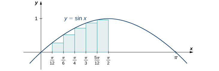
Let’s first look at the graph in Figure 5.15 to get a better idea of the area of interest.
英語のヒント
まず図5.15のグラフを見て、求めたい領域の形を把握しよう。
OpenStax, Rice University; Calculus Volume 1. · CC BY-NC-SA 4.0
Figure 5.15図 5.15
The graph of is divided into six regions:
のグラフの区間を六つに分ける。小区間の幅は である。
The intervals are and Note that is increasing on the interval so a left-endpoint approximation gives us the lower sum. A left-endpoint approximation is the Riemann sum We have
小区間は と である。 は区間 上で増加するので、左端近似で下和が得られる。左端近似に対応するリーマン和は である。したがって、