第11章カイ二乗分布

11.2 Goodness-of-Fit Test11.2　適合度検定

In this type of hypothesis test, you determine whether the data "fit" a particular distribution or not. For example, you may suspect your unknown data fit a binomial distribution. You use a chi-square test (meaning the distribution for the hypothesis test is chi-square) to determine if there is a fit or not. The null and the alternative hypotheses for this test may be written in sentences or may be stated as equations or inequalities.

英語のヒント

この種類の仮説検定では、データが特定の分布に「適合」するかどうかを調べる。例えば、分布が不明なデータが二項分布に適合するのではないかと考えることがある。適合するかどうかは、カイ二乗検定（仮説検定に用いる分布がカイ二乗分布であるという意味）で判断する。この検定の帰無仮説と対立仮説は、文章で書いても、等式や不等式で表してもよい。

The test statistic for a goodness-of-fit test is:

適合度検定の検定統計量は次のとおりである。

\underset{k}{Σ} \frac{{(O - E)}^{2}}{E}

where:

ここで、各記号は次を表す。

O = observed values (data)
O = 観測値（データ）
E = expected values (from theory)
E = 期待値（理論から求める）
k = the number of different data cells or categories
k = 異なるデータのセルまたはカテゴリーの数

The observed values are the data values and the expected values are the values you would expect to get if the null hypothesis were true. There are n terms of the form

\frac{{(O - E)}^{2}}{E}

英語のヒント

観測値とは実際のデータの値であり、期待値とは帰無仮説が正しいなら得られると予想される値である。

\frac{{(O - E)}^{2}}{E}

という形の項がn個ある。

The number of degrees of freedom is df = (number of categories – 1).

自由度はdf =（カテゴリーの数 − 1）である。

The goodness-of-fit test is almost always right-tailed. If the observed values and the corresponding expected values are not close to each other, then the test statistic can get very large and will be way out in the right tail of the chi-square curve.

英語のヒント

適合度検定は、ほとんどの場合、右片側検定である。観測値とそれに対応する期待値が互いに近くなければ、検定統計量は非常に大きくなり、カイ二乗曲線の右裾の遠い位置にくる。

Example 11.1例題 11.1

Absenteeism of college students from math classes is a major concern to math instructors because missing class appears to increase the drop rate. Suppose that a study was done to determine if the actual student absenteeism rate follows faculty perception. The faculty expected that a group of 100 students would miss class according to Table 11.1.

英語のヒント

大学生が数学の授業を欠席することは、数学の教員にとって大きな懸念である。欠席すると履修を取りやめる割合が高まるとみられるからだ。学生の実際の欠席状況が教員の認識に一致するかを調べる研究を行ったとする。教員は、100人の学生が表11.1のように欠席すると予想した。

Table 11.1表 11.1
Number of absences per term 1学期あたりの欠席回数	Expected number of students 予想される学生数
0–2	50
3–5	30
6–8	12
9–11	6
12+	2

A random survey across all mathematics courses was then done to determine the actual number (observed) of absences in a course. The chart in Table 11.2 displays the results of that survey.

次に、全数学科目を対象とした無作為調査で、1科目での実際の欠席回数（観測値）を調べた。表11.2は、その調査結果を示している。

Table 11.2表 11.2
Number of absences per term 1学期あたりの欠席回数	Actual number of students 実際の学生数
0–2	35
3–5	40
6–8	20
9–11	1
12+	4

Determine the null and alternative hypotheses needed to conduct a goodness-of-fit test.

適合度検定の実施に必要な帰無仮説と対立仮説を定めよう。

H₀: Student absenteeism fits faculty perception.

H₀：学生の欠席状況は教員の認識に適合する。

The alternative hypothesis is the opposite of the null hypothesis.

対立仮説は帰無仮説の反対である。

H_a: Student absenteeism does not fit faculty perception.

H_a：学生の欠席状況は教員の認識に適合しない。

a. Can you use the information as it appears in the charts to conduct the goodness-of-fit test?

a. 表に示された情報をそのまま使って、適合度検定を実施できるか。

Solution解き方

a. No. Notice that the expected number of absences for the "12+" entry is less than five (it is two). Combine that group with the "9–11" group to create new tables where the number of students for each entry are at least five. The new results are in Table 11.3 and Table 11.4.

英語のヒント

a. できない。「12回以上」の欄の期待度数が5未満（2）であることに注目しよう。この群を「9～11回」の群と合わせ、各欄の学生数が少なくとも5になるように新たな表を作る。新たな結果を表11.3と表11.4に示す。

Table 11.3表 11.3
Number of absences per term 1学期あたりの欠席回数	Expected number of students 予想される学生数
0–2	50
3–5	30
6–8	12
9+	8

Table 11.4表 11.4
Number of absences per term 1学期あたりの欠席回数	Actual number of students 実際の学生数
0–2	35
3–5	40
6–8	20
9+	5

b. What is the number of degrees of freedom (df)?

b. 自由度（df）はいくつか。

Solution解き方

b. There are four "cells" or categories in each of the new tables.

b. 新しい表には、それぞれ四つの「セル」、すなわちカテゴリーがある。

df = number of cells – 1 = 4 – 1 = 3

df = セルの数 − 1 = 4 − 1 = 3

Try Itやってみよう

A factory manager needs to understand how many products are defective versus how many are produced. The number of expected defects is listed in Table 11.5.

英語のヒント

工場の管理者は、生産された製品数に対して不良品がいくつあるかを把握する必要がある。予想される不良品数を表11.5に示す。

Table 11.5表 11.5
Number produced 生産数	Number defective 不良品数
0–100	5
101–200	6
201–300	7
301–400	8
401–500	10

A random sample was taken to determine the actual number of defects. Table 11.6 shows the results of the survey.

実際の不良品数を調べるため、無作為標本を抽出した。表11.6は調査結果を示している。

Table 11.6表 11.6
Number produced 生産数	Number defective 不良品数
0–100	5
101–200	7
201–300	8
301–400	9
401–500	11

State the null and alternative hypotheses needed to conduct a goodness-of-fit test, and state the degrees of freedom.

適合度検定に必要な帰無仮説と対立仮説、および自由度を示そう。

Example 11.2例題 11.2

Employers want to know which days of the week employees are absent in a five-day work week. Most employers would like to believe that employees are absent equally during the week. Suppose a random sample of 60 managers were asked on which day of the week they had the highest number of employee absences. The results were distributed as in Table 11.7. For the population of employees, do the days for the highest number of absences occur with equal frequencies during a five-day work week? Test at a 5% significance level.

英語のヒント

雇用主は、週5日勤務のうち、従業員がどの曜日に欠勤するかを知りたい。多くの雇用主は、各曜日に同じ程度の欠勤があると考えたいだろう。無作為に抽出した60人の管理者に、従業員の欠勤が最も多かったのは何曜日かを尋ねたとする。結果は表11.7のように分布した。従業員の母集団について、欠勤が最も多い曜日は、週5日の間に同じ度数で出現するだろうか。有意水準5%で検定しよう。

Day of the Week Employees were Most Absent従業員の欠勤が最も多かった曜日

Table 11.7表 11.7
	Monday 月曜日	Tuesday 火曜日	Wednesday 水曜日	Thursday 木曜日	Friday 金曜日
Number of Absences 欠勤数	15	12	9	9	15

Solution解き方

The null and alternative hypotheses are:

帰無仮説と対立仮説は次のとおりである。

H₀: The absent days occur with equal frequencies, that is, they fit a uniform distribution.
H₀：欠勤日は同じ度数で出現する。すなわち、一様分布に適合する。
H_a: The absent days occur with unequal frequencies, that is, they do not fit a uniform distribution.
H_a：欠勤日は異なる度数で出現する。すなわち、一様分布に適合しない。

If the absent days occur with equal frequencies, then, out of 60 absent days (the total in the sample: 15 + 12 + 9 + 9 + 15 = 60), there would be 12 absences on Monday, 12 on Tuesday, 12 on Wednesday, 12 on Thursday, and 12 on Friday. These numbers are the expected (E) values. The values in the table are the observed (O) values or data.

欠勤日が同じ度数で出現するなら、60件の欠勤日（標本の合計：15 + 12 + 9 + 9 + 15 = 60）のうち、月曜日が12件、火曜日が12件、水曜日が12件、木曜日が12件、金曜日が12件となるはずである。これらの数が期待値（E）である。表の値は観測値（O）、すなわちデータである。

This time, calculate the χ² test statistic by hand. Make a chart with the following headings and fill in the columns:

今回は、χ²検定統計量を手計算しよう。次の見出しを持つ表を作り、各列を埋めよう。

Expected (E) values (12, 12, 12, 12, 12)
期待値（E）（12, 12, 12, 12, 12）
Observed (O) values (15, 12, 9, 9, 15)
観測値（O）（15, 12, 9, 9, 15）
(O – E)
(O – E)²
$\frac{{(O – E)}^{2}}{E}$

Now add (sum) the last column. The sum is three. This is the χ² test statistic.

最後の列を足し合わせよう。合計は3になる。これがχ²検定統計量である。

To find the p-value, calculate P(χ² > 3). This test is right-tailed. (Use a computer or calculator to find the p-value. You should get p-value = 0.5578.)

p値を求めるには、P(χ² > 3)を計算する。この検定は右片側検定である。（コンピューターか電卓を使ってp値を求めよう。p値 = 0.5578となるはずである。）

The dfs are the number of cells – 1 = 5 – 1 = 4

自由度は、セルの数 − 1 = 5 − 1 = 4である。

Using the Calculator電卓の操作

Next, complete a graph like the following one with the proper labeling and shading. (You should shade the right tail.)

次に、以下のようなグラフに適切なラベルと陰影を加え、完成させよう。（右裾に陰影を付ける。）

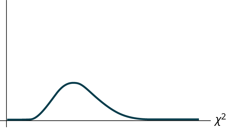
欠勤した曜日についての検定統計量を示す、書き込み前の非対称のカイ二乗曲線。 — Figure 11.5図 11.5

The decision is not to reject the null hypothesis.

帰無仮説を棄却しないと判断する。

Conclusion: At a 5% level of significance, from the sample data, there is not sufficient evidence to conclude that the absent days do not occur with equal frequencies.

英語のヒント

結論：有意水準5%では、標本データから、欠勤日が同じ度数で出現しないと結論する十分な証拠は得られない。

Using the Calculator電卓の操作

TI-83+ and some TI-84 calculators do not have a special program for the test statistic for the goodness-of-fit test. The next example Example 11.3 has the calculator instructions. The newer TI-84 calculators have in STAT TESTS the test Chi2 GOF. To run the test, put the observed values (the data) into a first list and the expected values (the values you expect if the null hypothesis is true) into a second list. Press STAT TESTS and Chi2 GOF. Enter the list names for the Observed list and the Expected list. Enter the degrees of freedom and press calculate or draw. Make sure you clear any lists before you start. To Clear Lists in the calculators: Go into STAT EDIT and arrow up to the list name area of the particular list. Press CLEAR and then arrow down. The list will be cleared. Alternatively, you can press STAT and press 4 (for ClrList). Enter the list name and press ENTER.

英語のヒント

TI-83+と一部のTI-84電卓には、適合度検定の検定統計量を求める専用プログラムがない。次の例11.3に電卓の操作手順を示す。新しいTI-84電卓では、STAT TESTSにChi2 GOFという検定がある。検定を実行するには、観測値（データ）を第1のリストに、期待値（帰無仮説が正しければ予想される値）を第2のリストに入力する。STAT TESTS、Chi2 GOFを押す。ObservedとExpectedに、それぞれのリスト名を入力する。自由度を入力し、calculateまたはdrawを押す。始める前に、使用するリストを必ず消去しておこう。電卓のリストを消去するには、STAT EDITに入り、上矢印で目的のリストの名前欄に移動する。CLEARを押してから下矢印を押すと、リストが消去される。別の方法として、STATを押して4（ClrList）を押し、リスト名を入力してENTERを押してもよい。

Try Itやってみよう

Teachers want to know which night each week their students are doing most of their homework. Most teachers think that students do homework equally throughout the week. Suppose a random sample of 56 students were asked on which night of the week they did the most homework. The results were distributed as in Table 11.8.

英語のヒント

教師たちは、生徒が1週間のどの夜に最も多く宿題をしているのかを知りたい。多くの教師は、生徒は1週間を通じて同じ程度に宿題をしていると考えている。無作為に抽出した56人の生徒に、1週間のどの夜に最も多く宿題をしたかを尋ねたとする。結果は表11.8のように分布した。

Table 11.8表 11.8
	Sunday 日曜日	Monday 月曜日	Tuesday 火曜日	Wednesday 水曜日	Thursday 木曜日	Friday 金曜日	Saturday 土曜日
Number of Students 生徒数	11	8	10	7	10	5	5

From the population of students, do the nights for the highest number of students doing the majority of their homework occur with equal frequencies during a week? What type of hypothesis test should you use?

生徒の母集団について、宿題の大部分を行う生徒数が最も多くなる夜は、1週間の間に同じ度数で出現するだろうか。どの種類の仮説検定を使うべきか。

Example 11.3例題 11.3

One study indicates that the number of streaming services that American families have is distributed (this is the given distribution for the American population) as in Table 11.9.

ある研究では、米国の家庭が利用している動画配信サービスの数は、表11.9のように分布しているという（これを米国の母集団について与えられた分布とする）。

Table 11.9表 11.9
Number of Streaming Services 動画配信サービスの数	Percent 百分率
0	10
1	16
2	55
3	11
4+	8

The table contains expected (E) percents.

この表には、予想される百分率（E）が示されている。

A random sample of 600 families in the far western United States resulted in the data in Table 11.10.

米国最西部の600世帯を無作為に抽出したところ、表11.10のデータが得られた。

Table 11.10表 11.10
Number of Streaming Services 動画配信サービスの数	Frequency 度数
0	66
1	119
2	340
3	60
4+	15
	Total = 600 合計 = 600

The table contains observed (O) frequency values.

この表には、観測度数（O）が示されている。

At the 1% significance level, does it appear that the distribution "number of streaming services" of far western United States families is different from the distribution for the American population as a whole?

有意水準1%で、米国最西部の家庭の「動画配信サービスの数」の分布は、米国全体の母集団の分布と異なるといえるか。

Solution解き方

This problem asks you to test whether the far western United States families distribution fits the distribution of the American families. This test is always right-tailed.

この問題では、米国最西部の家庭の分布が、米国の家庭の分布に適合するかを検定する。この検定は常に右片側検定である。

The first table contains expected percentages. To get expected (E) frequencies, multiply the percentage by 600. The expected frequencies are shown in Table 11.11.

最初の表には、予想される百分率が示されている。期待度数（E）を得るには、その百分率に600を掛ける。期待度数を表11.11に示す。

Table 11.11表 11.11
Number of Streaming Services 動画配信サービスの数	Percent 百分率	Expected Frequency 期待度数
0	10	(0.10)(600) = 60
1	16	(0.16)(600) = 96
2	55	(0.55)(600) = 330
3	11	(0.11)(600) = 66
over 3 3より多い	8	(0.08)(600) = 48

Therefore, the expected frequencies are 60, 96, 330, 66, and 48. In the TI calculators, you can let the calculator do the math. For example, instead of 60, enter 0.10*600.

したがって、期待度数は60、96、330、66、48となる。TI電卓では、その計算を電卓に任せられる。例えば、60の代わりに0.10*600と入力する。

H₀: The "number of streaming services" distribution of far western United States families is the same as the "number of streaming services" distribution of the American population.

H₀：米国最西部の家庭の「動画配信サービスの数」の分布は、米国の母集団の「動画配信サービスの数」の分布と同じである。

H_a: The "number of streaming services" distribution of far western United States families is different from the "number of streaming services" distribution of the American population.

H_a：米国最西部の家庭の「動画配信サービスの数」の分布は、米国の母集団の「動画配信サービスの数」の分布と異なる。

Distribution for the test:

χ_{4}^{2}

where df = (the number of cells) – 1 = 5 – 1 = 4.

検定に用いる分布：

χ_{4}^{2}

。ここでdf =（セルの数）− 1 = 5 − 1 = 4である。

Calculate the test statistic: χ2 = 29.65

検定統計量を計算する：χ2 = 29.65

Graph:

グラフ：

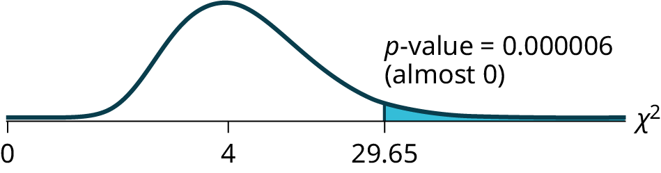
横軸に0、4、29.65が記された非対称のカイ二乗曲線。4は曲線の頂点に対応する。29.65から曲線まで垂直線が上に延び、その右側の領域に陰影が付いている。陰影部分の面積がp値に等しい。 — Figure 11.6図 11.6

Probability statement: p-value = P(χ² > 29.65) = 0.000006

確率の式：p値 = P(χ² > 29.65) = 0.000006

Compare α and the p-value:

αとp値を比較する。

α = 0.01
p-value = 0.000006
p値 = 0.000006

So, α > p-value.

したがって、α > p値である。

Make a decision: Since α > p-value, reject H_o.

判断：α > p値なので、H_oを棄却する。

This means you reject the belief that the distribution for the far western states is the same as that of the American population as a whole.

英語のヒント

これは、最西部の州の分布が米国全体の母集団の分布と同じだという考えを棄却することを意味する。

Conclusion: At the 1% significance level, from the data, there is sufficient evidence to conclude that the "number of streaming services" distribution for the far western United States is different from the "number of streaming services" distribution for the American population as a whole.

結論：有意水準1%では、このデータから、米国最西部の「動画配信サービスの数」の分布が、米国全体の母集団の「動画配信サービスの数」の分布と異なると結論する十分な証拠が得られる。

Using the Calculator電卓の操作

Press STAT and ENTER. Make sure to clear lists L1, L2, and L3 if they have data in them (see the note at the end of Example 11.2). Into L1, put the observed frequencies 66, 119, 340, 60, 15. Into L2, put the expected frequencies .10*600, .16*600, .55*600, .11*600, .08*600. Arrow over to list L3 and up to the name area "L3". Enter (L1-L2)^2/L2 and ENTER. Press 2nd QUIT. Press 2nd LIST and arrow over to MATH. Press 5. You should see "sum" (Enter L3). Rounded to 2 decimal places, you should see 29.65. Press 2nd DISTR. Press 7 or Arrow down to 7:χ2cdf and press ENTER. Enter (29.65,1E99,4). Rounded to four places, you should see 5.77E-6 = .000006 (rounded to six decimal places), which is the p-value.

STAT、ENTERを押す。L1、L2、L3にデータが入っている場合は、必ず消去しておく（例11.2の末尾の注を参照）。L1に観測度数66, 119, 340, 60, 15を入力する。L2に期待度数.10*600, .16*600, .55*600, .11*600, .08*600を入力する。右矢印でL3に移り、上矢印で名前欄「L3」に移動する。(L1-L2)^2/L2を入力してENTERを押す。2nd、QUITを押す。2nd、LISTを押し、横矢印でMATHへ移動する。5を押すと「sum」が表示されるはずである（L3を入力する）。小数第2位までに丸めると29.65になるはずである。2nd、DISTRを押す。7を押すか、下矢印で7:χ2cdfに移動してENTERを押す。(29.65,1E99,4)を入力する。小数第4位までに丸めると5.77E-6、すなわち.000006（小数第6位までに丸めた値）が表示されるはずである。これがp値である。

The newer TI-84 calculators have in STAT TESTS the test Chi2 GOF. To run the test, put the observed values (the data) into a first list and the expected values (the values you expect if the null hypothesis is true) into a second list. Press STAT TESTS and Chi2 GOF. Enter the list names for the Observed list and the Expected list. Enter the degrees of freedom and press calculate or draw. Make sure you clear any lists before you start.

新しいTI-84電卓では、STAT TESTSにChi2 GOFという検定がある。検定を実行するには、観測値（データ）を第1のリストに、期待値（帰無仮説が正しければ予想される値）を第2のリストに入力する。STAT TESTS、Chi2 GOFを押す。ObservedとExpectedに、それぞれのリスト名を入力する。自由度を入力し、calculateまたはdrawを押す。始める前に、使用するリストを必ず消去しておこう。

Try Itやってみよう

The expected percentage of the number of pets students have in their homes is distributed (this is the given distribution for the student population of the United States) as in Table 11.12.

生徒が家庭で飼っているペットの数について、予想される百分率は表11.12のように分布している（これを米国の生徒の母集団について与えられた分布とする）。

Table 11.12表 11.12
Number of Pets ペットの数	Percent 百分率
0	18
1	25
2	30
3	18
4+	9

A random sample of 1,000 students from the Eastern United States resulted in the data in Table 11.13.

米国東部の生徒1,000人を無作為に抽出したところ、表11.13のデータが得られた。

Table 11.13表 11.13
Number of Pets ペットの数	Frequency 度数
0	210
1	240
2	320
3	140
4+	90

At the 1% significance level, does it appear that the distribution “number of pets” of students in the Eastern United States is different from the distribution for the United States student population as a whole? What is the p-value?

有意水準1%で、米国東部の生徒の「ペットの数」の分布は、米国全体の生徒の母集団の分布と異なるといえるか。p値はいくつか。

Example 11.4例題 11.4

Suppose you flip two coins 100 times. The results are 20 HH, 27 HT, 30 TH, and 23 TT. Are the coins fair? Test at a 5% significance level.

英語のヒント

2枚の硬貨を100回投げたとする。結果はHHが20回、HTが27回、THが30回、TTが23回だった。硬貨に偏りはないだろうか。有意水準5%で検定しよう。

Solution解き方

This problem can be set up as a goodness-of-fit problem. The sample space for flipping two fair coins is {HH, HT, TH, TT}. Out of 100 flips, you would expect 25 HH, 25 HT, 25 TH, and 25 TT. This is the expected distribution. The question, "Are the coins fair?" is the same as saying, "Does the distribution of the coins (20 HH, 27 HT, 30 TH, 23 TT) fit the expected distribution?"

この問題は適合度の問題として設定できる。偏りのない2枚の硬貨を投げるときの標本空間は{HH, HT, TH, TT}である。100回投げれば、HHが25回、HTが25回、THが25回、TTが25回と予想される。これが期待される分布である。「硬貨に偏りはないか」という問いは、「硬貨の結果の分布（HHが20回、HTが27回、THが30回、TTが23回）は期待される分布に適合するか」と同じである。

Random Variable: Let X = the number of heads in one flip of the two coins. X takes on the values 0, 1, 2. (There are 0, 1, or 2 heads in the flip of two coins.) Therefore, the number of cells is three. Since X = the number of heads, the observed frequencies are 20 (for two heads), 57 (for one head), and 23 (for zero heads or both tails). The expected frequencies are 25 (for two heads), 50 (for one head), and 25 (for zero heads or both tails). This test is right-tailed.

確率変数：Xを、2枚の硬貨を1回投げたときに表が出る枚数とする。Xは0、1、2の値をとる。（2枚の硬貨を投げると、表の枚数は0、1、2のいずれかになる。）したがって、セルの数は3である。Xは表の枚数なので、観測度数は20（表が2枚）、57（表が1枚）、23（表が0枚、すなわち両方裏）である。期待度数は25（表が2枚）、50（表が1枚）、25（表が0枚、すなわち両方裏）である。この検定は右片側検定である。

H₀: The coins are fair.

H₀：硬貨に偏りはない。

H_a: The coins are not fair.

H_a：硬貨には偏りがある。

Distribution for the test:

χ_{2}^{2}

where df = 3 – 1 = 2.

検定に用いる分布：

χ_{2}^{2}

。ここでdf = 3 − 1 = 2である。

Calculate the test statistic: χ² = 2.14

検定統計量を計算する：χ² = 2.14

Graph:

グラフ：

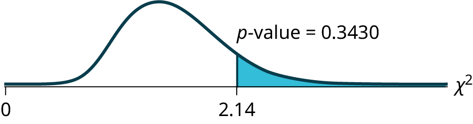
横軸に0と2.14が記された非対称のカイ二乗曲線。2.14から曲線まで垂直線が上に延び、その右側の領域に陰影が付いている。陰影部分の面積がp値に等しい。 — Figure 11.7図 11.7

Probability statement: p-value = P(χ² > 2.14) = 0.3430

確率の式：p値 = P(χ² > 2.14) = 0.3430

Compare α and the p-value:

αとp値を比較する。

α = 0.05
p-value = 0.3430
p値 = 0.3430

α < p-value.

α < p値。

Make a decision: Since α < p-value, do not reject H₀.

判断：α < p値なので、H₀を棄却しない。

Conclusion: There is insufficient evidence to conclude that the coins are not fair.

結論：硬貨に偏りがあると結論する十分な証拠はない。

Using the Calculator電卓の操作

Press STAT and ENTER. Make sure you clear lists L1, L2, and L3 if they have data in them. Into L1, put the observed frequencies 20, 57, 23. Into L2, put the expected frequencies 25, 50, 25. Arrow over to list L3 and up to the name area "L3". Enter (L1-L2)^2/L2 and ENTER. Press 2nd QUIT. Press 2nd LIST and arrow over to MATH. Press 5. You should see "sum".Enter L3. Rounded to two decimal places, you should see 2.14. Press 2nd DISTR. Arrow down to 7:χ2cdf (or press 7). Press ENTER. Enter 2.14,1E99,2). Rounded to four places, you should see .3430, which is the p-value.

STAT、ENTERを押す。L1、L2、L3にデータがある場合は、必ず消去しておく。L1に観測度数20, 57, 23を入力する。L2に期待度数25, 50, 25を入力する。横矢印でL3へ、上矢印で名前欄「L3」へ移動する。(L1-L2)^2/L2を入力し、ENTERを押す。2nd、QUITを押す。2nd、LISTを押し、横矢印でMATHへ移動する。5を押すと「sum」が表示されるはずである。L3を入力する。小数第2位までに丸めると2.14になるはずである。2nd、DISTRを押し、下矢印で7:χ2cdfに移動する（または7を押す）。ENTERを押し、2.14,1E99,2)を入力する。小数第4位までに丸めると、p値である.3430が表示されるはずである。

Try Itやってみよう

Students in a social studies class hypothesize that the literacy rates across the world for every region are 82%. Table 11.14 shows the actual literacy rates across the world broken down by region. What are the test statistic and the degrees of freedom?

英語のヒント

社会科の生徒たちが、世界のどの地域でも識字率は82%であるという仮説を立てた。表11.14は、世界の実際の識字率を地域別に示している。検定統計量と自由度はいくつか。

Table 11.14表 11.14
MDG Region MDG地域区分	Adult Literacy Rate (%) 成人識字率（%）
Developed Regions 先進地域	99.0
Commonwealth of Independent States 独立国家共同体	99.5
Northern Africa 北アフリカ	67.3
Sub-Saharan Africa サハラ以南アフリカ	62.5
Latin America and the Caribbean ラテンアメリカ・カリブ海地域	91.0
Eastern Asia 東アジア	93.8
Southern Asia 南アジア	61.9
South-Eastern Asia 東南アジア	91.9
Western Asia 西アジア	84.5
Oceania オセアニア	66.4

第11章カイ二乗分布

11.2 Goodness-of-Fit Test11.2 適合度検定

Day of the Week Employees were Most Absent従業員の欠勤が最も多かった曜日

11.2 Goodness-of-Fit Test11.2　適合度検定