第2章極限

2.2 The Limit of a Function2.2　関数の極限

Learning Objectives学習目標

Using correct notation, describe the limit of a function.
正しい記号を使って、関数の極限を表す。
Use a table of values to estimate the limit of a function or to identify when the limit does not exist.
値の表を使って関数の極限を推定し、極限が存在しない場合を見分ける。
Use a graph to estimate the limit of a function or to identify when the limit does not exist.
グラフを使って関数の極限を推定し、極限が存在しない場合を見分ける。
Define one-sided limits and provide examples.
片側極限を定義し、例を挙げる。
Explain the relationship between one-sided and two-sided limits.
片側極限と両側極限の関係を説明する。
Using correct notation, describe an infinite limit.
正しい記号を使って、無限大への発散を表す。
Define a vertical asymptote.
垂直漸近線を定義する。

The concept of a limit or limiting process, essential to the understanding of calculus, has been around for thousands of years. In fact, early mathematicians used a limiting process to obtain better and better approximations of areas of circles. Yet, the formal definition of a limit—as we know and understand it today—did not appear until the late 19th century. We therefore begin our quest to understand limits, as our mathematical ancestors did, by using an intuitive approach. At the end of this chapter, armed with a conceptual understanding of limits, we examine the formal definition of a limit.

英語のヒント

微積分の理解に欠かせない極限、あるいは極限操作の考え方は、何千年も前から存在していた。実際、古代の数学者は極限操作を用いて、円の面積をより正確に近似していた。しかし、現在私たちが理解しているような極限の厳密な定義が現れたのは、19世紀後半になってからである。そこで、数学の先人たちと同じように、まず直感的な方法で極限の理解を始めよう。この章の最後では、極限の概念を理解したうえで、厳密な定義を調べる。

We begin our exploration of limits by taking a look at the graphs of the functions

次の関数のグラフを見て、極限の探究を始めよう。

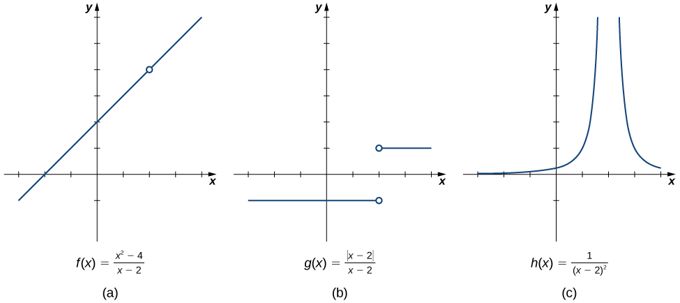
f (x) = \frac{x^{2} - 4}{x - 2}, g (x) = \frac{| x - 2 |}{x - 2}, and h (x) = \frac{1}{{(x - 2)}^{2}},

f (x) = \frac{x^{2} - 4}{x - 2}, g (x) = \frac{| x - 2 |}{x - 2}, および h (x) = \frac{1}{{(x - 2)}^{2}}

which are shown in Figure 2.12. In particular, let’s focus our attention on the behavior of each graph at and around

x = 2 .

これらのグラフを図2.12に示す。特に、

x = 2

とその周辺での各グラフの振る舞いに注目しよう。

3つの関数のグラフ。第1のf(x)=(x²−4)/(x−2)は、x切片が(−2,0)の直線で、(2,4)だけが白丸になっている。第2のg(x)=|x−2|/(x−2)は、x>2ではy=1、x<2ではy=−1の2本の水平な半直線で、端点(2,1)と(2,−1)は白丸である。第3のh(x)=1/(x−2)²は常に正で、漸近線y=0とx=2を持つ。原文の代替説明にある軸・座標の取り違えを、式に合わせて訂正している。 — Figure 2.12図 2.12
These graphs show the behavior of three different functions around $x = 2 .$
3つの異なる関数について、 $x = 2$ 付近での振る舞いを示したグラフ。

Each of the three functions is undefined at

x = 2,

but if we make this statement and no other, we give a very incomplete picture of how each function behaves in the vicinity of

x = 2 .

To express the behavior of each graph in the vicinity of 2 more completely, we need to introduce the concept of a limit.

英語のヒント

この3つの関数は、いずれも

x = 2

では定義されていない。しかし、それだけを述べても、

x = 2

付近で各関数がどう振る舞うかは、ほとんど伝わらない。2の近くでのグラフの様子をより十分に表すには、極限という概念が必要になる。

Intuitive Definition of a Limit極限の直感的な定義

Let’s first take a closer look at how the function

f (x) = (x^{2} - 4) / (x - 2)

behaves around

x = 2

in Figure 2.12. As the values of x approach 2 from either side of 2, the values of

y = f (x)

approach 4. Mathematically, we say that the limit of

f (x)

as x approaches 2 is 4. Symbolically, we express this limit as

英語のヒント

まず図2.12で、関数

f (x) = (x^{2} - 4) / (x - 2)

が

x = 2

付近でどう振る舞うか、詳しく見よう。xを2の左右どちらから近づけても、

y = f (x)

は4に近づく。数学では、これを「xが2に近づくときの

f (x)

の極限は4である」という。記号では、次のように表す。

lim_{x \to 2} f (x) = 4 .

lim_{x \to 2} f (x) = 4

From this very brief informal look at one limit, let’s start to develop an intuitive definition of the limit. We can think of the limit of a function at a number a as being the one real number L that the functional values approach as the x-values approach a, provided such a real number L exists. Stated more carefully, we have the following definition:

英語のヒント

1つの極限を大まかに見たところで、極限の直感的な定義を考えよう。ある数aでの関数の極限とは、xの値をaに近づけるとき、関数の値が近づくただ1つの実数Lだと考えられる。そのような実数Lが存在する場合の話である。より丁寧に述べると、次の定義になる。

Definition定義

Let

f (x)

be a function defined at all values in an open interval containing a, with the possible exception of a itself, and let L be a real number. If all values of the function

f (x)

approach the real number L as the values of

x (\neq a)

approach the number a, then we say that the limit of

f (x)

as x approaches a is L. (More succinct, as x gets closer to a,

f (x)

gets closer and stays close to L.) Symbolically, we express this idea as

英語のヒント

aを含むある開区間内のすべての値で、関数

f (x)

が定義されているとする。ただし、aそのものでは定義されていなくてもよい。また、Lを実数とする。

x (\neq a)

をaに近づけたとき、関数

f (x)

の値がすべて実数Lに近づくなら、「xがaに近づくときの

f (x)

の極限はLである」という。簡潔にいえば、xがaに近づくにつれ、

f (x)

がLに近づき、その近くにとどまるということである。記号では、次のように表す。

lim_{x \to a} f (x) = L .

lim_{x \to a} f (x) = L

(2.3)

We can estimate limits by constructing tables of functional values and by looking at their graphs. This process is described in the following Problem-Solving Strategy.

関数の値の表を作ったり、グラフを調べたりすることで、極限を推定できる。その手順を、次の解法の指針にまとめる。

Evaluating a Limit Using a Table of Functional Values関数の値の表から極限を求める

To evaluate

lim_{x \to a} f (x),

we begin by completing a table of functional values. We should choose two sets of x-values—one set of values approaching a and less than a, and another set of values approaching a and greater than a. Table 2.1 demonstrates what your tables might look like.

lim_{x \to a} f (x)

を求めるには、まず関数の値の表を作る。xの値は2組選び、1組はaより小さい側からaに近づけ、もう1組はaより大きい側からaに近づける。表2.1は、そのような表の例である。

Table of Functional Values for $lim_{x \to a} f (x)$ $lim_{x \to a} f (x)$ を求めるための関数値の表

Table 2.1表 2.1
x	$f (x)$	x	$f (x)$
$a - 0.1$	$f (a - 0.1)$	$a + 0.1$	$f (a + 0.1)$
$a - 0.01$	$f (a - 0.01)$	$a + 0.01$	$f (a + 0.01)$
$a - 0.001$	$f (a - 0.001)$	$a + 0.001$	$f (a + 0.001)$
$a - 0.0001$	$f (a - 0.0001)$	$a + 0.0001$	$f (a + 0.0001)$
Use additional values as necessary. 必要に応じて、さらに値を加える。		Use additional values as necessary. 必要に応じて、さらに値を加える。

Next, let’s look at the values in each of the $f (x)$ columns and determine whether the values seem to be approaching a single value as we move down each column. In our columns, we look at the sequence $f (a - 0.1), f (a - 0.01), f (a - 0.001) ., f (a - 0.0001),$ and so on, and $f (a + 0.1), f (a + 0.01), f (a + 0.001), f (a + 0.0001),$ and so on. (Note: Although we have chosen the x-values $a \pm 0.1, a \pm 0.01, a \pm 0.001, a \pm 0.0001,$ and so forth, and these values will probably work nearly every time, on very rare occasions we may need to modify our choices.)
次に、 $f (x)$ の各列を下へ読み進め、その値が1つの値に近づいているように見えるかを調べる。ここでは、 $f (a - 0.1), f (a - 0.01), f (a - 0.001) ., f (a - 0.0001)$ …という列と、 $f (a + 0.1), f (a + 0.01), f (a + 0.001), f (a + 0.0001)$ …という列を調べる。ここで選んだxの値は $a \pm 0.1, a \pm 0.01, a \pm 0.001, a \pm 0.0001$ …であり、ほとんどの場合はこの選び方でうまくいく。ただし、ごくまれに、別の値を選ぶ必要がある。
If both columns approach a common y-value L, we state $lim_{x \to a} f (x) = L .$ We can use the following strategy to confirm the result obtained from the table or as an alternative method for estimating a limit.
両方の列が同じyの値Lに近づくなら、 $lim_{x \to a} f (x) = L$ と判断する。表から得た結果を確かめるため、あるいは別の推定方法として、次の方法を使える。
Using a graphing calculator or computer software that allows us to graph functions, we can plot the function $f (x),$ making sure the functional values of $f (x)$ for x-values near a are in our window. We can use the trace feature to move along the graph of the function and watch the y-value readout as the x-values approach a. If the y-values approach L as our x-values approach a from both directions, then $lim_{x \to a} f (x) = L .$ We may need to zoom in on our graph and repeat this process several times.
英語のヒント
関数のグラフを描ける電卓やコンピューターソフトを使って、 $f (x)$ を描く。その際、aに近いxの値に対する $f (x)$ の値が、表示範囲内に入るようにする。トレース機能でグラフ上を移動し、xをaに近づけたときのyの表示値を観察する。xを左右のどちらからaに近づけてもyがLに近づくなら、 $lim_{x \to a} f (x) = L$ である。グラフを拡大して、この操作を何度か繰り返す必要があるかもしれない。

We apply this Problem-Solving Strategy to compute a limit in Example 2.4.

例題2.4では、この解法の指針を使って極限を求める。

Example 2.4例題 2.4

Evaluating a Limit Using a Table of Functional Values 1関数の値の表から極限を求める(1)

Evaluate

lim_{x \to 0} \frac{sin x}{x}

using a table of functional values.

関数の値の表を使って、

lim_{x \to 0} \frac{sin x}{x}

を求めなさい。

Solution解き方

We have calculated the values of

f (x) = (sin x) / x

for the values of x listed in Table 2.2.

表2.2に示すxの値について、

f (x) = (sin x) / x

の値を計算した。

Table of Functional Values for $lim_{x \to 0} \frac{sin x}{x}$ $lim_{x \to 0} \frac{sin x}{x}$ を求めるための関数値の表

Table 2.2表 2.2
x	$\frac{sin x}{x}$	x	$\frac{sin x}{x}$
−0.1	0.998334166468	0.1	0.998334166468
−0.01	0.999983333417	0.01	0.999983333417
−0.001	0.999999833333	0.001	0.999999833333
−0.0001	0.999999998333	0.0001	0.999999998333

Note: The values in this table were obtained using a calculator and using all the places given in the calculator output.

この表の数値は電卓で求め、表示された桁をすべて用いている。

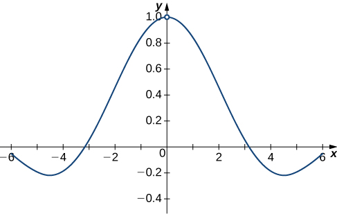
As we read down each

\frac{(sin x)}{x}

column, we see that the values in each column appear to be approaching one. Thus, it is fairly reasonable to conclude that

lim_{x \to 0} \frac{sin x}{x} = 1 .

A calculator or computer-generated graph of

f (x) = \frac{(sin x)}{x}

would be similar to that shown in Figure 2.13, and it confirms our estimate.

英語のヒント

\frac{(sin x)}{x}

の各列を下へ読むと、どちらの列の値も1に近づいているように見える。したがって、

lim_{x \to 0} \frac{sin x}{x} = 1

と結論づけるのは十分もっともらしい。電卓やコンピューターで

f (x) = \frac{(sin x)}{x}

を描くと、図2.13のようなグラフが得られ、この推定を裏づけている。

区間[−6,6]でのf(x)=sin(x)/xのグラフ。x=0では関数は未定義だが、グラフはy=1に近づく。x軸との交点はx=−πとx=πにある。原文の代替説明で混同されているxとyを訂正している。 — Figure 2.13図 2.13
The graph of $f (x) = (sin x) / x$ confirms the estimate from Table 2.2.
$f (x) = (sin x) / x$ のグラフは、表2.2からの推定を裏づけている。

Example 2.5例題 2.5

Evaluating a Limit Using a Table of Functional Values 2関数の値の表から極限を求める(2)

Evaluate

lim_{x \to 4} \frac{\sqrt{x} - 2}{x - 4}

using a table of functional values.

関数の値の表を使って、

lim_{x \to 4} \frac{\sqrt{x} - 2}{x - 4}

を求めなさい。

Solution解き方

As before, we use a table—in this case, Table 2.3—to list the values of the function for the given values of x.

前と同じように、指定されたxの値に対する関数の値を表にまとめる。ここでは表2.3を用いる。

Table of Functional Values for $lim_{x \to 4} \frac{\sqrt{x} - 2}{x - 4}$ $lim_{x \to 4} \frac{\sqrt{x} - 2}{x - 4}$ を求めるための関数値の表

Table 2.3表 2.3
x	$\frac{\sqrt{x} - 2}{x - 4}$	x	$\frac{\sqrt{x} - 2}{x - 4}$
3.9	0.251582341869	4.1	0.248456731317
3.99	0.25015644562	4.01	0.24984394501
3.999	0.250015627	4.001	0.249984377
3.9999	0.250001563	4.0001	0.249998438
3.99999	0.25000016	4.00001	0.24999984

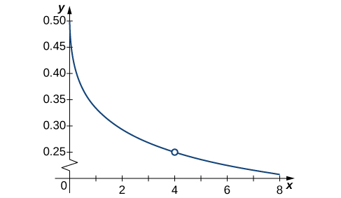
After inspecting this table, we see that the functional values less than 4 appear to be decreasing toward 0.25 whereas the functional values greater than 4 appear to be increasing toward 0.25. We conclude that

lim_{x \to 4} \frac{\sqrt{x} - 2}{x - 4} = 0.25 .

We confirm this estimate using the graph of

f (x) = \frac{\sqrt{x} - 2}{x - 4}

shown in Figure 2.14.

表を見ると、xが4より小さい側では関数の値が0.25へ向かって減少し、xが4より大きい側では0.25へ向かって増加しているように見える。したがって、

lim_{x \to 4} \frac{\sqrt{x} - 2}{x - 4} = 0.25

と結論づける。図2.14の

f (x) = \frac{\sqrt{x} - 2}{x - 4}

のグラフも、この推定を裏づける。

区間[0,8]でのf(x)=(√x−2)/(x−4)のグラフ。x=4に白丸があり、そこでは未定義である。曲線はx=0の値1/2から減少し、x=4では1/4に近づく。原文の代替説明の「y軸が漸近線」という記述は、この式には当てはまらない。 — Figure 2.14図 2.14
The graph of $f (x) = \frac{\sqrt{x} - 2}{x - 4}$ confirms the estimate from Table 2.3.
$f (x) = \frac{\sqrt{x} - 2}{x - 4}$ のグラフは、表2.3からの推定を裏づけている。

At this point, we see from Example 2.4 and Example 2.5 that it may be just as easy, if not easier, to estimate a limit of a function by inspecting its graph as it is to estimate the limit by using a table of functional values. In Example 2.6, we evaluate a limit exclusively by looking at a graph rather than by using a table of functional values.

英語のヒント

例題2.4と例題2.5から、グラフを調べて極限を推定する方法は、関数の値の表を使う方法より簡単な場合もあり、少なくとも同じくらい簡単だと分かる。例題2.6では、値の表を使わず、グラフを見るだけで極限を求める。

Example 2.6例題 2.6

Evaluating a Limit Using a Graphグラフから極限を求める

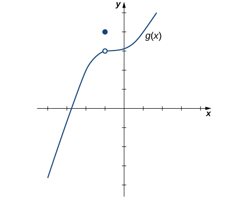
For

g (x)

shown in Figure 2.15, evaluate

lim_{x \to −1} g (x) .

図2.15に示す

g (x)

について、

lim_{x \to −1} g (x)

を求めなさい。

関数g(x)の曲線のグラフ。第2象限の点(−1,3)が白丸になっており、その1単位上の点(−1,4)に黒丸がある。 — Figure 2.15図 2.15
The graph of $g (x)$ includes one value not on a smooth curve.
$g (x)$ のグラフには、滑らかな曲線から外れた値が1つある。

Solution解き方

Despite the fact that

g (−1) = 4,

as the x-values approach −1 from either side, the

g (x)

values approach 3. Therefore,

lim_{x \to −1} g (x) = 3 .

Note that we can determine this limit without even knowing the algebraic expression of the function.

英語のヒント

g (−1) = 4

であるにもかかわらず、xを左右どちらから−1に近づけても、

g (x)

の値は3に近づく。したがって、

lim_{x \to −1} g (x) = 3

である。関数を表す代数式が分からなくても、この極限は求められる。

Based on Example 2.6, we make the following observation: It is possible for the limit of a function to exist at a point, and for the function to be defined at this point, but the limit of the function and the value of the function at the point may be different.

英語のヒント

例題2.6から、次のことが分かる。ある点で関数の極限が存在し、しかもその点で関数が定義されていても、極限の値とその点での関数の値が異なる場合がある。

Looking at a table of functional values or looking at the graph of a function provides us with useful insight into the value of the limit of a function at a given point. However, these techniques rely too much on guesswork. We eventually need to develop alternative methods of evaluating limits. These new methods are more algebraic in nature and we explore them in the next section; however, at this point we introduce two special limits that are foundational to the techniques to come.

英語のヒント

関数の値の表やグラフを見ると、ある点での極限の値を考えるうえで役に立つ。しかし、これらの方法は推測に頼りすぎている。いずれは、別の方法で極限を求める必要がある。次の節では、より代数的な方法を調べる。その前に、これからの手法の基礎になる、2つの特別な極限を紹介する。

We can make the following observations about these two limits.

この2つの極限について、次のように考えられる。

For the first limit, observe that as x approaches a, so does $f (x),$ because $f (x) = x .$ Consequently, $lim_{x \to a} x = a .$
第1の極限では、xがaに近づくと、 $f (x)$ もaに近づく。 $f (x) = x$ だからである。したがって、 $lim_{x \to a} x = a$ となる。
For the second limit, consider Table 2.4.
第2の極限については、表2.4を考えよう。

Table of Functional Values for $lim_{x \to a} c = c$ $lim_{x \to a} c = c$ の関数値の表

Table 2.4表 2.4
x	$f (x) = c$	x	$f (x) = c$
$a - 0.1$	c	$a + 0.1$	c
$a - 0.01$	c	$a + 0.01$	c
$a - 0.001$	c	$a + 0.001$	c
$a - 0.0001$	c	$a + 0.0001$	c

Observe that for all values of x (regardless of whether they are approaching a), the values

f (x)

remain constant at c. We have no choice but to conclude

lim_{x \to a} c = c .

英語のヒント

xがaに近づいているかどうかにかかわらず、どのxでも

f (x)

の値はcのままである。したがって、

lim_{x \to a} c = c

と結論づけられる。

第2章極限

2.2 The Limit of a Function2.2 関数の極限

Learning Objectives学習目標

Intuitive Definition of a Limit極限の直感的な定義

Evaluating a Limit Using a Table of Functional Values 1関数の値の表から極限を求める(1)

Table of Functional Values for limx→0sinxxlimx→0sinxxを求めるための関数値の表

Evaluating a Limit Using a Table of Functional Values 2関数の値の表から極限を求める(2)

Table of Functional Values for limx→4x−2x−4limx→4x−2x−4を求めるための関数値の表

Evaluating a Limit Using a Graphグラフから極限を求める

Table of Functional Values for limx→ac=climx→ac=cの関数値の表

2.2 The Limit of a Function2.2　関数の極限

Table of Functional Values for $lim_{x \to 0} \frac{sin x}{x}$ $lim_{x \to 0} \frac{sin x}{x}$ を求めるための関数値の表

Table of Functional Values for $lim_{x \to 4} \frac{\sqrt{x} - 2}{x - 4}$ $lim_{x \to 4} \frac{\sqrt{x} - 2}{x - 4}$ を求めるための関数値の表

Table of Functional Values for $lim_{x \to a} c = c$ $lim_{x \to a} c = c$ の関数値の表