第13章F分布と一元配置分散分析

References参考文献

“MLB Vs. Division Standings – 2012.” Available online at http://espn.go.com/mlb/standings/_/year/2012/type/vs-division/order/true.

「MLB Vs. Division Standings – 2012」（MLB地区内対戦順位、2012年）。オンライン：http://espn.go.com/mlb/standings/_/year/2012/type/vs-division/order/true。

Chapter Review章の復習

The F test for the equality of two variances rests heavily on the assumption of normal distributions. The test is unreliable if this assumption is not met. If both distributions are normal, then the ratio of the two sample variances is distributed as an F statistic, with numerator and denominator degrees of freedom that are one less than the samples sizes of the corresponding two groups. A test of two variances hypothesis test determines if two variances are the same. The distribution for the hypothesis test is the F distribution with two different degrees of freedom.

英語のヒント

二つの分散が等しいかどうかのF検定は、正規分布の仮定に強く依存する。この仮定が満たされなければ、検定は信頼できない。両方の分布が正規分布なら、二つの標本分散の比はF統計量として分布し、分子と分母の自由度は、それぞれ対応する群の標本の大きさより1小さい。二つの分散の仮説検定は、二つの分散が同じかどうかを判断する。この仮説検定に用いる分布は、異なる二つの自由度を持つF分布である。

Assumptions:仮定：

The populations from which the two samples are drawn are normally distributed.
二つの標本を抽出した母集団が、正規分布に従う。
The two populations are independent of each other.
二つの母集団が互いに独立である。

Formula Review公式の復習

F has the distribution F ~ F(n₁ – 1, n₂ – 1)

Fは、F ~ F(n₁ – 1, n₂ – 1)という分布に従う。

F =

\frac{\frac{s_{1}^{2}}{σ_{1}^{2}}}{\frac{s_{2}^{2}}{σ_{2}^{2}}}

If σ₁ = σ₂, then F =

\frac{s_{1}^{2}}{s_{2}^{2}}

σ₁ = σ₂ならば、F =

\frac{s_{1}^{2}}{s_{2}^{2}}

である。

Exercises 59–60練習問題 59–60

Use the following information to answer the next two exercises. There are two assumptions that must be true in order to perform an F test of two variances.

次の二つの練習問題には、以下の情報を用いる。二つの分散のF検定を行うには、二つの仮定が満たされていなければならない。

Exercise 59問題 59

Name one assumption that must be true.

満たされるべき仮定を一つ挙げよ。

Solution解き方

The populations from which the two samples are drawn are normally distributed.

二つの標本を抽出した母集団が、正規分布に従う。

Exercise 60問題 60

What is the other assumption that must be true?

満たされるべきもう一つの仮定は何か。

Exercises 61–67練習問題 61–67

Use the following information to answer the next five exercises. Two coworkers commute from the same building. They are interested in whether or not there is any variation in the time it takes them to drive to work. They each record their times for 20 commutes. The first worker’s times have a variance of 12.1. The second worker’s times have a variance of 16.9. The first worker thinks that he is more consistent with his commute times. Test the claim at the 10% level. Assume that commute times are normally distributed.

英語のヒント

次の五つの練習問題には、以下の情報を用いる。同じ建物から通勤する二人の同僚が、職場まで車で行く時間のばらつきに違いがあるかどうかに関心を持っている。それぞれが20回の通勤時間を記録した。1人目の時間の分散は12.1、2人目は16.9だった。1人目は、自分の通勤時間の方が安定していると考えている。この主張を10%水準で検定せよ。通勤時間は正規分布に従うと仮定する。

Exercise 61問題 61

State the null and alternative hypotheses.

帰無仮説と対立仮説を示す。

Solution解き方

H₀: σ₁ = σ₂

H_a: σ₁ < σ₂

または

H₀:

σ_{1}^{2} = σ_{2}^{2}

H_a:

σ_{1}^{2} < σ_{2}^{2}

Exercise 62問題 62

What is s₁ in this problem?

この問題のs₁はいくつか。

Exercise 63問題 63

What is s₂ in this problem?

この問題のs₂はいくつか。

Solution解き方

4.11

Exercise 64問題 64

What is n?

nはいくつか。

Exercise 65問題 65

What is the F statistic?

F統計量はいくつか。

Solution解き方

0.7159

Exercise 66問題 66

What is the p-value?

p値はいくつか。

Exercise 67問題 67

Is the claim accurate?

その主張は正しいか。

Solution解き方

No, at the 10% level of significance, we do not reject the null hypothesis and state that the data do not show that the variation in drive times for the first worker is less than the variation in drive times for the second worker.

正しいとはいえない。有意水準10%では帰無仮説を棄却しない。このデータは、1人目の通勤時間のばらつきが、2人目の通勤時間のばらつきより小さいことを示していない。

Exercises 68–71練習問題 68–71

Use the following information to answer the next four exercises. Two students are interested in whether or not there is variation in their test scores for math class. There are 15 total math tests they have taken so far. The first student’s grades have a standard deviation of 38.1. The second student’s grades have a standard deviation of 22.5. The second student thinks his scores are more consistent.

次の四つの練習問題には、以下の情報を用いる。二人の学生が、数学の試験の点数のばらつきに違いがあるかどうかに関心を持っている。これまでに受けた数学の試験は計15回である。1人目の点数の標準偏差は38.1、2人目は22.5だった。2人目は、自分の点数の方が安定していると考えている。

Exercise 68問題 68

State the null and alternative hypotheses.

帰無仮説と対立仮説を示す。

Exercise 69問題 69

What is the F Statistic?

F統計量はいくつか。

Solution解き方

2.8674

Exercise 70問題 70

What is the p-value?

p値はいくつか。

Exercise 71問題 71

At the 5% significance level, do we reject the null hypothesis?

有意水準5%で、帰無仮説を棄却するか。

Solution解き方

Reject the null hypothesis. There is enough evidence to say that the variance of the grades for the first student is higher than the variance in the grades for the second student.

帰無仮説を棄却する。1人目の点数の分散が2人目より大きいといえる、十分な証拠がある。

Exercises 72–74練習問題 72–74

Use the following information to answer the next three exercises. Two cyclists are comparing the variances of their overall paces going uphill. Each cyclist records their speeds going up 35 hills. The first cyclist has a variance of 23.8 and the second cyclist has a variance of 32.1. The cyclists want to see if their variances are the same or different. Assume that commute times are normally distributed.

英語のヒント

次の三つの練習問題には、以下の情報を用いる。二人の自転車乗りが、上り坂を走る全体的なペースの分散を比較している。それぞれが35の坂を上る速度を記録した。1人目の分散は23.8、2人目は32.1だった。二人は、自分たちの分散が同じか異なるかを知りたい。通勤時間は正規分布に従うと仮定する。

Exercise 72問題 72

State the null and alternative hypotheses.

帰無仮説と対立仮説を示す。

Exercise 73問題 73

What is the F Statistic?

F統計量はいくつか。

Solution解き方

0.7414

Exercise 74問題 74

At the 5% significance level, what can we say about the cyclists’ variances?

有意水準5%で、二人の自転車乗りの分散について何がいえるか。

Homework宿題

Exercises 75–83練習問題 75–83

Exercise 75問題 75

Three students, Linda, Tuan, and Javier, are given five laboratory rats each for a nutritional experiment. Each rat’s weight is recorded in grams. Linda feeds her rats Formula A, Tuan feeds his rats Formula B, and Javier feeds his rats Formula C. At the end of a specified time period, each rat is weighed again and the net gain in grams is recorded.

栄養実験のために、リンダ、トゥアン、ハビエルの3人の学生に、それぞれ実験用ラット5匹を渡す。各ラットの体重をグラム単位で記録する。リンダは飼料A、トゥアンは飼料B、ハビエルは飼料Cを、自分のラットに与える。一定の期間が過ぎたら各ラットの体重を再び量り、正味の増加量をグラム単位で記録する。

Table 13.31表 13.31
Linda's rats リンダのラット	Tuan's rats トゥアンのラット	Javier's rats ハビエルのラット
43.5	47.0	51.2
39.4	40.5	40.9
41.3	38.9	37.9
46.0	46.3	45.0
38.2	44.2	48.6

Determine whether or not the variance in weight gain is statistically the same among Javier’s and Linda’s rats. Test at a significance level of 10%.

ハビエルとリンダのラットで、体重増加量の分散が統計的に同じかどうかを判断せよ。有意水準10%で検定する。

Solution解き方

$H_{0} : σ_{1}^{2} = σ_{2}^{2}$
$H_{a} : σ_{1}^{2} \neq σ_{1}^{2}$
df(num) = 4; df(denom) = 4
df(num) = 4、df(denom) = 4
F_{4, 4}
3.00
2(0.1563) = 0.3126. Using the TI-83+/84+ function 2-SampFtest, you get the test statistic as 2.9986 and p-value directly as 0.3127. If you input the lists in a different order, you get a test statistic of 0.3335 but the p-value is the same because this is a two-tailed test.
2(0.1563) = 0.3126。TI-83+/84+の2-SampFtest関数を使うと、検定統計量2.9986と、p値0.3127が直接得られる。リストを別の順序で入力すると検定統計量は0.3335になるが、両側検定なのでp値は同じである。
Answers may vary.
解答はさまざまである。
Decision: Do not reject the null hypothesis; Conclusion: There is insufficient evidence to conclude that the variances are different.
判断：帰無仮説を棄却しない。結論：分散が異なると結論するための十分な証拠はない。

Exercise 76問題 76

A grassroots group opposed to a proposed increase in the gas tax claimed that the increase would hurt working-class people the most, since they commute the farthest to work. Suppose that the group randomly surveyed 24 individuals and asked them their daily one-way commuting mileage. The results are as follows.

ガソリン税の増税案に反対する草の根団体は、労働者階級の人々は通勤距離が最も長いため、増税による被害も最も大きいと主張した。この団体が24人を無作為に調査し、毎日の片道通勤距離をマイル単位で尋ねたとする。結果は次のとおりである。

Table 13.32表 13.32
working-class 労働者階級	professional (middle incomes) 専門職（中所得）	professional (wealthy) 専門職（富裕層）
17.8	16.5	8.5
26.7	17.4	6.3
49.4	22.0	4.6
9.4	7.4	12.6
65.4	9.4	11.0
47.1	2.1	28.6
19.5	6.4	15.4
51.2	13.9	9.3

Determine whether or not the variance in mileage driven is statistically the same among the working class and professional (middle income) groups. Use a 5% significance level.

労働者階級と専門職（中所得）の群で、運転距離の分散が統計的に同じかどうかを判断せよ。有意水準は5%とする。

Use the following information to answer the next two exercises. Table 13.33 lists the number of pages in four different types of magazines.

次の二つの練習問題には、以下の情報を用いる。表13.33は、異なる四種類の雑誌のページ数を示す。

Table 13.33表 13.33
home decorating インテリア	news ニュース	health 健康	computer コンピューター
172	87	82	104
286	94	153	136
163	123	87	98
205	106	103	207
197	101	96	146

Exercise 77問題 77

Which two magazine types do you think have the same variance in length?

どの二種類の雑誌のページ数の分散が同じだと思うか。

Exercise 78問題 78

Which two magazine types do you think have different variances in length?

どの二種類の雑誌のページ数の分散が異なると思うか。

Solution解き方

The answers may vary. Sample answer: Home decorating magazines and news magazines have different variances.

解答はさまざまである。解答例：インテリア雑誌とニュース雑誌は分散が異なる。

Exercise 79問題 79

Is the variance for the amount of money, in dollars, that shoppers spend on Saturdays at the mall the same as the variance for the amount of money that shoppers spend on Sundays at the mall? Suppose that the Table 13.34 shows the results of a study.

土曜日に買い物客がショッピングモールで使う金額（ドル）の分散は、日曜日に使う金額の分散と同じか。表13.34に調査結果を示す。

Table 13.34表 13.34
Saturday 土曜日	Sunday 日曜日	Saturday 土曜日	Sunday 日曜日
75	44	62	137
18	58	0	82
150	61	124	39
94	19	50	127
62	99	31	141
73	60	118	73
	89

Exercise 80問題 80

Are the variances for incomes on the East Coast and the West Coast the same? Suppose that Table 13.35 shows the results of a study. Income is shown in thousands of dollars. Assume that both distributions are normal. Use a level of significance of 0.05.

東海岸と西海岸の収入の分散は同じか。表13.35に調査結果を示す。収入の単位は千ドルである。両方の分布は正規分布に従うと仮定する。有意水準は0.05とする。

Table 13.35表 13.35
East 東部	West 西部
38	71
47	126
30	42
82	51
75	44
52	90
115	88
67

Solution解き方

H₀: = $σ_{1}^{2}$ = $σ_{2}^{2}$
H_a: $σ_{1}^{2}$ ≠ $σ_{1}^{2}$
df(n) = 7, df(d) = 6
df(n) = 7、df(d) = 6
F_7,6
0.8117
0.7825
Answers may vary.
解答はさまざまである。
1. Alpha: 0.05
  α：0.05
2. Decision: Do not reject the null hypothesis.
  判断：帰無仮説を棄却しない。
3. Reason for decision: p-value > alpha
  判断の理由：p値 > α
4. Conclusion: There is not sufficient evidence to conclude that the variances are different.
  結論：分散が異なると結論するための十分な証拠はない。

Exercise 81問題 81

Thirty men in college were taught a method of finger tapping. They were randomly assigned to three groups of ten, with each receiving one of three doses of caffeine: 0 mg, 100 mg, 200 mg. This is approximately the amount in no, one, or two cups of coffee. Two hours after ingesting the caffeine, the men had the rate of finger tapping per minute recorded. The experiment was double blind, so neither the recorders nor the students knew which group they were in. Does caffeine affect the rate of tapping, and if so how?

英語のヒント

男子大学生30人に、指を繰り返し動かしてたたく方法を教えた。10人ずつの三つの群に無作為に割り当て、カフェインを0 mg、100 mg、200 mgのいずれかの量だけ摂取させた。これは、およそコーヒー0杯、1杯、2杯に含まれる量に当たる。摂取の2時間後に、1分間あたり指を動かした回数を記録した。実験は二重盲検であり、記録者も学生も、学生がどの群に属するかを知らなかった。カフェインは指を動かす速さに影響するか。影響するなら、どのような影響か。

Here are the data:

データを以下に示す。

Table 13.36表 13.36
0 mg	100 mg	200 mg	0 mg	100 mg	200 mg
242	248	246	245	246	248
244	245	250	248	247	252
247	248	248	248	250	250
242	247	246	244	246	248
246	243	245	242	244	250

Exercise 82問題 82

King Manuel I, Komnenus ruled the Byzantine Empire from Constantinople (Istanbul) during the years 1145 to 1180 A.D. The empire was very powerful during his reign, but declined significantly afterwards. Coins minted during his era were found in Cyprus, an island in the eastern Mediterranean Sea. Nine coins were from his first coinage, seven from the second, four from the third, and seven from a fourth. These spanned most of his reign. We have data on the silver content of the coins:

英語のヒント

マヌエル1世コムネノスは、西暦1145年から1180年にかけて、コンスタンティノープル（イスタンブール）からビザンツ帝国を統治した。帝国は彼の治世中には非常に強大だったが、その後大きく衰退した。彼の時代に鋳造された硬貨が、地中海東部の島キプロスで発見された。最初の鋳造期の硬貨が9枚、2期目が7枚、3期目が4枚、4期目が7枚で、治世の大半を覆う。硬貨の銀含有量のデータを以下に示す。

Table 13.37表 13.37
First Coinage 第1鋳造期	Second Coinage 第2鋳造期	Third Coinage 第3鋳造期	Fourth Coinage 第4鋳造期
5.9	6.9	4.9	5.3
6.8	9.0	5.5	5.6
6.4	6.6	4.6	5.5
7.0	8.1	4.5	5.1
6.6	9.3		6.2
7.7	9.2		5.8
7.2	8.6		5.8
6.9
6.2

Did the silver content of the coins change over the course of Manuel’s reign?

マヌエルの治世の間に、硬貨の銀含有量は変化したか。

Here are the means and variances of each coinage. The data are unbalanced.

各鋳造期の平均と分散を以下に示す。このデータは釣り合っていない。

Table 13.38表 13.38
	First 第1期	Second 第2期	Third 第3期	Fourth 第4期
Mean 平均	6.7444	8.2429	4.875	5.6143
Variance 分散	0.2953	1.2095	0.2025	0.1314

Solution解き方

Here is a strip chart of the silver content of the coins:

硬貨の銀含有量のストリップチャートを以下に示す。

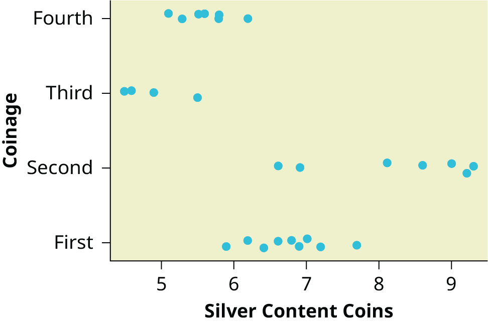
与えられたデータを表す散布図。横軸は「硬貨の銀含有量」で、5から9までを示す。縦軸は「鋳造期」で、第1期、第2期、第3期、第4期の区分がある。 — Figure 13.10図 13.10

While there are differences in spread, it is not unreasonable to use ANOVA techniques. Here is the completed ANOVA table:

広がりには違いがあるものの、分散分析の手法を用いることは不合理ではない。完成した分散分析表を以下に示す。

Table 13.39表 13.39
Source of Variation 変動の要因	Sum of Squares (SS) 平方和（SS）	Degrees of Freedom (df) 自由度（df）	Mean Square (MS) 平均平方（MS）	F
Factor (Between) 因子（群間）	37.748	4 – 1 = 3	12.5825	26.272
Error (Within) 誤差（群内）	11.015	27 – 4 = 23	0.4789
Total 合計	48.763	27 – 1 = 26

P(F > 26.272) = 0;

Reject the null hypothesis for any alpha. There is sufficient evidence to conclude that the mean silver content among the four coinages are different. From the strip chart, it appears that the first and second coinages had higher silver contents than the third and fourth.

どのαに対しても帰無仮説を棄却する。四つの鋳造期の平均銀含有量が異なると結論するための、十分な証拠がある。ストリップチャートからは、第1期と第2期の硬貨の方が、第3期と第4期より銀含有量が高かったと考えられる。

Exercise 83問題 83

The American League and the National League of Major League Baseball are each divided into three divisions: East, Central, and West. Many years, fans talk about some divisions being stronger (having better teams) than other divisions. This may have consequences for the postseason. For instance, in a certain year Tampa Bay won 90 games and did not play in the postseason, while Detroit won only 88 and did play in the postseason. This may have been an oddity, but is there good evidence that in this year, the American League divisions were significantly different in overall records? Use the following data to test whether the mean number of wins per team in the three American League divisions were the same or not. Note that the data are not balanced, as two divisions had five teams, while one had only four.

英語のヒント

メジャーリーグベースボールのアメリカンリーグとナショナルリーグは、それぞれ東・中・西の三つの地区に分かれている。ある地区は他の地区より強い、つまり良いチームがそろっている、という話がファンの間でよく出る。これはポストシーズンにも影響しうる。例えば、ある年にはタンパベイが90勝してもポストシーズンに進めず、デトロイトは88勝で進んだ。これは例外的な出来事だったのかもしれないが、その年のアメリカンリーグの地区間で、全体的な成績に有意な差があったという十分な証拠はあるだろうか。次のデータを使い、アメリカンリーグの三地区で、1チームあたりの平均勝利数が同じかどうかを検定せよ。二つの地区には5チーム、残る一つには4チームしかないため、データは釣り合っていないことに注意する。

Table 13.40表 13.40
Division 地区	Team チーム	Wins 勝利数
East 東部	NY Yankees ニューヨーク・ヤンキース	95
East 東部	Baltimore ボルチモア	93
East 東部	Tampa Bay タンパベイ	90
East 東部	Toronto トロント	73
East 東部	Boston ボストン	69

Table 13.41表 13.41
Division 地区	Team チーム	Wins 勝利数
Central 中部	Detroit デトロイト	88
Central 中部	Chicago Sox シカゴ・ソックス	85
Central 中部	Kansas City カンザスシティ	72
Central 中部	Cleveland クリーブランド	68
Central 中部	Minnesota ミネソタ	66

Table 13.42表 13.42
Division 地区	Team チーム	Wins 勝利数
West 西部	Oakland オークランド	94
West 西部	Texas テキサス	93
West 西部	LA Angels ロサンゼルス・エンゼルス	89
West 西部	Seattle シアトル	75

Solution解き方

Here is a stripchart of the number of wins for the 14 teams in the AL for the 2012 season.

2012年シーズンのアメリカンリーグ14チームの勝利数について、ストリップチャートを示す。

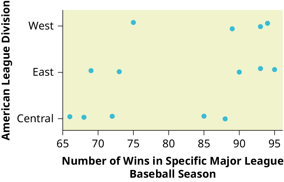
与えられたデータを表す散布図。横軸は「2012年メジャーリーグベースボールの勝利数」で、65から95までを示す。縦軸は「アメリカンリーグの地区」で、中部、東部、西部の区分がある。 — Figure 13.11図 13.11

While the spread seems similar, there may be some question about the normality of the data, given the wide gaps in the middle near the 0.500 mark of 82 games (teams play 162 games each season in MLB). However, one-way ANOVA is robust.

英語のヒント

広がりは同程度に見えるが、中央の82勝、勝率0.500付近に大きな空白があるので、データの正規性には多少疑問があるかもしれない（MLBでは、各チームが1シーズン162試合を行う）。しかし、一元配置分散分析は頑健である。

Here is the ANOVA table for the data:

このデータの分散分析表を以下に示す。

Table 13.43表 13.43
Source of Variation 変動の要因	Sum of Squares (SS) 平方和（SS）	Degrees of Freedom (df) 自由度（df）	Mean Square (MS) 平均平方（MS）	F
Factor (Between) 因子（群間）	344.16	3 – 1 = 2	172.08
Error (Within) 誤差（群内）	1,219.55	14 – 3 = 11	110.87	1.5521
Total 合計	1,563.71	14 – 1 = 13

P(F > 1.5521) = 0.2548
Since the p-value is so large, there is not good evidence against the null hypothesis of equal means. We decline to reject the null hypothesis. Thus, for 2012, there is not any have any good evidence of a significant difference in mean number of wins between the divisions of the American League.

英語のヒント

P(F > 1.5521) = 0.2548。p値がこれほど大きいので、平均が等しいという帰無仮説に反する十分な証拠はない。帰無仮説を棄却しない。したがって2012年については、アメリカンリーグの地区間で平均勝利数に有意な差があるという、十分な証拠はない。

0 mg	100 mg	200 mg	0 mg	100 mg	200 mg
242	248	246	245	246	248
244	245	250	248	247	252
247	248	248	248	250	250
242	247	246	244	246	248
246	243	245	242	244	250

First Coinage 第1鋳造期	Second Coinage 第2鋳造期	Third Coinage 第3鋳造期	Fourth Coinage 第4鋳造期
5.9	6.9	4.9	5.3
6.8	9.0	5.5	5.6
6.4	6.6	4.6	5.5
7.0	8.1	4.5	5.1
6.6	9.3		6.2
7.7	9.2		5.8
7.2	8.6		5.8
6.9
6.2

0 mg	100 mg	200 mg	0 mg	100 mg	200 mg
242	248	246	245	246	248
244	245	250	248	247	252
247	248	248	248	250	250
242	247	246	244	246	248
246	243	245	242	244	250

First Coinage 第1鋳造期	Second Coinage 第2鋳造期	Third Coinage 第3鋳造期	Fourth Coinage 第4鋳造期
5.9	6.9	4.9	5.3
6.8	9.0	5.5	5.6
6.4	6.6	4.6	5.5
7.0	8.1	4.5	5.1
6.6	9.3		6.2
7.7	9.2		5.8
7.2	8.6		5.8
6.9
6.2

0 mg	100 mg	200 mg	0 mg	100 mg	200 mg
242	248	246	245	246	248
244	245	250	248	247	252
247	248	248	248	250	250
242	247	246	244	246	248
246	243	245	242	244	250

First Coinage 第1鋳造期	Second Coinage 第2鋳造期	Third Coinage 第3鋳造期	Fourth Coinage 第4鋳造期
5.9	6.9	4.9	5.3
6.8	9.0	5.5	5.6
6.4	6.6	4.6	5.5
7.0	8.1	4.5	5.1
6.6	9.3		6.2
7.7	9.2		5.8
7.2	8.6		5.8
6.9
6.2