第2章一次元の運動Motion in One Dimension原書 p.55–96
2.3 Position vs. Time Graphs2.3 位置–時間グラフ
SECTION LEARNING OBJECTIVES By the end of this section, you will be able to do the following:• Explain the meaning of slope in position vs. time graphs• Solve problems using position vs. time graphs
この節の学習目標 この節を終えると、次のことができるようになる。・位置–時間グラフにおける傾きの意味を説明する・位置–時間グラフを使って問題を解く
Section Key Termsこの節の重要語
dependent variableindependent variabletangent
従属変数独立変数接線
Graphing Position as a Function of Time位置を時間の関数としてグラフに描く
A graph, like a picture, is worth a thousand words. Graphs not only contain numerical information, they also reveal relationships between physical quantities. In this section, we will investigate kinematics by analyzing graphs of position over time.
グラフは、絵と同じように、多くの言葉を費やすよりも物事を端的に伝えられる。グラフは数値の情報を含むだけでなく、物理量どうしの関係も見せてくれる。この節では、位置の時間変化のグラフを分析することで運動学を調べる。
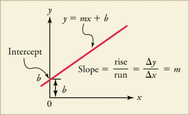
Graphs in this text have perpendicular axes, one horizontal and the other vertical. When two physical quantities are plotted against each other, the horizontal axis is usually considered the independent variable, and the vertical axis is the dependent variable. In algebra, you would have referred to the horizontal axis as the x-axis and the vertical axis as the y-axis. As in Figure 2.10, a straight-line graph has the general form .
本書のグラフは、水平と鉛直の直交する二軸を持つ。二つの物理量を互いに対して描くとき、ふつう水平軸を独立変数、鉛直軸を従属変数とする。代数では、水平軸をx軸、鉛直軸をy軸と呼んでいただろう。図2.10のように、直線のグラフは一般にの形をとる。
Here m is the slope, defined as the rise divided by the run (as seen in the figure) of the straight line. The letter b is the y-intercept which is the point at which the line crosses the vertical, y-axis. In terms of a physical situation in the real world, these quantities will take on a specific significance, as we will see below. (Figure 2.10.)
ここでmは傾きで、直線の(図に示したとおり)縦の変化を横の変化で割ったものと定義される。bはy切片で、直線が鉛直なy軸と交わる点である。現実の物理的な状況では、これらの量は特定の意味を持つことになる。以下で見ていこう(図2.10)。
In physics, time is usually the independent variable. Other quantities, such as displacement, are said to depend upon it. A graph of position versus time, therefore, would have position on the vertical axis (dependent variable) and time on the horizontal axis (independent variable). In this case, to what would the slope and y-intercept refer? Let’s look back at our original example when studying distance and displacement.
物理ではふつう時間が独立変数である。変位などの他の量は、時間に依存すると言われる。したがって位置–時間グラフでは、鉛直軸に位置(従属変数)、水平軸に時間(独立変数)をとる。この場合、傾きとy切片は何を指すことになるのか。道のりと変位を学んだときの最初の例に戻ってみよう。
The drive to school was 5 km from home. Let’s assume it took 10 minutes to make the drive and that your parent was driving at a constant velocity the whole time. The position versus time graph for this section of the trip would look like that shown in Figure 2.11.
学校までの道のりは家から5 kmだった。運転に10分かかり、その間ずっと親が一定の速度で運転していたとしよう。この区間の位置–時間グラフは、図2.11のようになる。
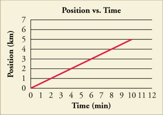
As we said before, d0 = 0 because we call home our O and start calculating from there. In Figure 2.11, the line starts at d = 0, as well. This is the b in our equation for a straight line. Our initial position in a position versus time graph is always the place where the graph crosses the x-axis at t = 0. What is the slope? The rise is the change in position, (i.e., displacement) and the run is the change in time. This relationship can also be written
先に述べたとおり、家を原点Oと呼びそこから計算を始めるので、d0 = 0である。図2.11でも、線はd = 0から始まっている。これが直線の式のbにあたる。位置–時間グラフにおける初めの位置は、t = 0における縦軸の値、すなわち縦軸との切片である。では傾きは何か。縦の変化は位置の変化(すなわち変位)、横の変化は時間の変化である。この関係は次のようにも書ける。
This relationship was how we defined average velocity. Therefore, the slope in a d versus t graph, is the average velocity.
この関係こそ、平均速度を定義したものだった。したがって、d–tグラフの傾きは平均速度である。
TIPS FOR SUCCESS Sometimes, as is the case where we graph both the trip to school and the return trip, the behavior of the graph looks different during different time intervals. If the graph looks like a series of straight lines, then you can calculate the average velocity for each time interval by looking at the slope. If you then want to calculate the average velocity for the entire trip, you can do a weighted average.
学習のポイント 学校までの行程と帰りの行程の両方をグラフにする場合のように、時間区間ごとにグラフの特徴が違って見えることがある。グラフが何本かの直線をつないだ形に見えるなら、各区間の傾きを見ることで、その区間の平均速度を計算できる。そのうえで全行程の平均速度を計算したければ、重み付き平均をとればよい。
Let’s look at another example. Figure 2.12 shows a graph of position versus time for a jet-powered car on a very flat dry lake bed in Nevada.
別の例を見よう。図2.12は、ネバダ州のきわめて平らな干上がった湖底を走るジェット推進車の、位置–時間グラフである。
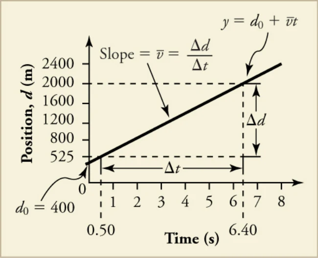
Using the relationship between dependent and independent variables, we see that the slope in the graph in Figure 2.12 is average velocity, vavg and the intercept is displacement at time zero—that is, d0. Substituting these symbols into y = mx + b gives
従属変数と独立変数の関係を使えば、図2.12のグラフの傾きが平均速度vavgであり、切片は時刻0における変位、すなわちd0であることがわかる。これらの記号を y = mx + b に代入すると、次が得られる。
or
すなわち、
Thus a graph of position versus time gives a general relationship among displacement, velocity, and time, as well as giving detailed numerical information about a specific situation. From the figure we can see that the car has a position of 400 m at t = 0 s, 650 m at t = 1.0 s, and so on. And we can learn about the object’s velocity, as well.
このように位置–時間グラフは、変位・速度・時間の間の一般的な関係を与えると同時に、特定の状況についての詳しい数値の情報も与えてくれる。図から、この車はt = 0 sで位置400 m、t = 1.0 sで650 m、というふうに読み取れる。そして物体の速度についても知ることができる。
SNAP LAB身近な実験Graphing Motion運動をグラフにする
In this activity, you will release a ball down a ramp and graph the ball’s displacement vs. time.
この活動では、斜面にボールを転がし、ボールの変位と時間のグラフを描く。
• Choose an open location with lots of space to spread out so there is less chance for tripping or falling due to rolling balls.
・ボールが転がってつまずいたり転んだりする危険が少ないよう、広く散らばれる開けた場所を選ぶこと。
• 1 ball• 1 board• 2 or 3 books• 1 stopwatch• 1 tape measure• 6 pieces of masking tape• 1 piece of graph paper• 1 pencil
・ボール1個・板1枚・本2〜3冊・ストップウォッチ1個・巻き尺1本・マスキングテープ6片・方眼紙1枚・鉛筆1本
Procedure手順
1. Build a ramp by placing one end of the board on top of the stack of books. Adjust location, as necessary, until there is no obstacle along the straight line path from the bottom of the ramp until at least the next 3 m.2. Mark distances of 0.5 m, 1.0 m, 1.5 m, 2.0 m, 2.5 m, and 3.0 m from the bottom of the ramp. Write the distances on the tape.3. Have one person take the role of the experimenter. This person will release the ball from the top of the ramp. If the ball does not reach the 3.0 m mark, then increase the incline of the ramp by adding another book. Repeat this Step as necessary.4. Have the experimenter release the ball. Have a second person, the timer, begin timing the trial once the ball reaches the bottom of the ramp and stop the timing once the ball reaches 0.5 m. Have a third person, the recorder, record the time in a data table.5. Repeat Step 4, stopping the times at the distances of 1.0 m, 1.5 m, 2.0 m, 2.5 m, and 3.0 m from the bottom of the ramp.6. Use your measurements of time and the displacement to make a position vs. time graph of the ball’s motion.7. Repeat Steps 4 through 6, with different people taking on the roles of experimenter, timer, and recorder. Do you get the same measurement values regardless of who releases the ball, measures the time, or records the result? Discuss possible causes of discrepancies, if any.
1. 板の一端を積んだ本の上に置いて斜面を作る。斜面の下端から少なくとも3 m先まで、直線の経路上に障害物がないよう、必要に応じて場所を調整する。2. 斜面の下端から0.5 m、1.0 m、1.5 m、2.0 m、2.5 m、3.0 mの距離に印を付ける。距離をテープに書いておく。3. 一人が実験係になる。この人が斜面の上端からボールを離す。ボールが3.0 mの印まで届かないなら、本を足して斜面の傾きを大きくする。必要なだけこの手順を繰り返す。4. 実験係にボールを離してもらう。二人目の計時係が、ボールが斜面の下端に達したところで計時を始め、0.5 mに達したところで止める。三人目の記録係が、時間を表に記録する。5. 手順4を繰り返し、斜面の下端から1.0 m、1.5 m、2.0 m、2.5 m、3.0 mの各距離で計時を止める。6. 測った時間と変位を使って、ボールの運動の位置–時間グラフを作る。7. 実験係・計時係・記録係を交代して、手順4から6を繰り返す。誰がボールを離し、誰が計時し、誰が記録しても、同じ測定値が得られるだろうか。食い違いがあれば、その原因になりうるものを話し合おう。
True or False: The average speed of the ball will be less than the average velocity of the ball.a. Trueb. False
正誤問題:ボールの平均の速さは、ボールの平均速度より小さくなる。a. 正b. 誤
Solving Problems Using Position vs. Time Graphs So how do we use graphs to solve for things we want to know like velocity?
位置–時間グラフを使って問題を解く では、速度のような知りたいものを求めるのに、グラフをどう使えばよいのだろうか。
Using Position–Time Graph to Calculate Average Velocity: Jet Car Find the average velocity of the car whose position is graphed in Figure 1.13. Strategy
位置–時間グラフを使って平均速度を計算する:ジェット車 図1.13に位置が描かれている車の平均速度を求めよ。 方針
The slope of a graph of d vs. t is average velocity, since slope equals rise over run.
傾きは縦の変化を横の変化で割ったものなので、d–tグラフの傾きは平均速度である。
Since the slope is constant here, any two points on the graph can be used to find the slope.
ここでは傾きが一定なので、グラフ上のどの2点を使って傾きを求めてもよい。
Solution解答
1. Choose two points on the line. In this case, we choose the points labeled on the graph: (6.4 s, 2000 m) and (0.50 s, 525 m). (Note, however, that you could choose any two points.)2. Substitute the d and t values of the chosen points into the equation. Remember in calculating change (Δ) we always use final value minus initial value.
1. 直線上の2点を選ぶ。ここではグラフに印の付いた2点(6.4 s, 2000 m)と(0.50 s, 525 m)を選ぶ(ただし、どの2点を選んでもよい)。2. 選んだ点のdとtの値を式に代入する。変化量(Δ)を計算するときは、つねに終わりの値から初めの値を引くことを忘れずに。
Discussion考察
This is an impressively high land speed (900 km/h, or about 560 mi/h): much greater than the typical highway speed limit of 27 m/s or 96 km/h, but considerably shy of the record of 343 m/s or 1,234 km/h, set in 1997.
これは驚くほど速い地上速度(900 km/h、およそ560 mi/h)である。よくある高速道路の制限速度27 m/s(96 km/h)よりはるかに速いが、1997年に記録された343 m/s(1,234 km/h)にはかなり及ばない。
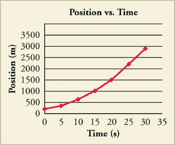
But what if the graph of the position is more complicated than a straight line? What if the object speeds up or turns around and goes backward? Can we figure out anything about its velocity from a graph of that kind of motion? Let’s take another look at the jet-powered car. The graph in Figure 2.13 shows its motion as it is getting up to speed after starting at rest. Time starts at zero for this motion (as if measured with a stopwatch), and the displacement and velocity are initially 200 m and 15 m/s, respectively.
だが、位置のグラフが直線より込み入っていたらどうなるか。物体が速くなったり、向きを変えて戻ってきたりしたら。そういう運動のグラフから、速度について何か読み取れるだろうか。もう一度ジェット推進車を見てみよう。図2.13のグラフは、静止から動き出して速さを上げていく間の運動を示している。この運動では(ストップウォッチで測るように)時間は0から始まり、変位と速度は初め、それぞれ200 mと15 m/sである。
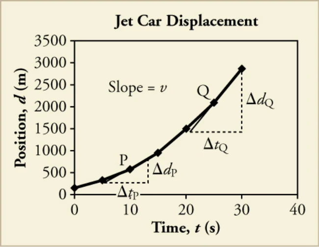

The graph of position versus time in Figure 2.13 is a curve rather than a straight line. The slope of the curve becomes steeper as time progresses, showing that the velocity is increasing over time. The slope at any point on a position-versus-time graph is the instantaneous velocity at that point. It is found by drawing a straight line tangent to the curve at the point of interest and taking the slope of this straight line. Tangent lines are shown for two points in Figure 2.13. The average velocity is the net displacement divided by the time traveled.
図2.13の位置–時間グラフは直線ではなく曲線である。時間が進むにつれて曲線の傾きは急になり、速度が時間とともに増していることを示している。位置–時間グラフ上の任意の点における傾きが、その点における瞬間速度である。それは、関心のある点で曲線に接する直線を引き、その直線の傾きをとることで求められる。図2.13には2点について接線が示してある。平均速度は、正味の変位を移動時間で割ったものである。
Using Position–Time Graph to Calculate Average Velocity: Jet Car, Take Two Calculate the instantaneous velocity of the jet car at a time of 25 s by finding the slope of the tangent line at point Q in Figure 2.13.Strategy
位置–時間グラフを使って平均速度を計算する:ジェット車、その2 図2.13の点Qにおける接線の傾きを求めることで、時刻25 sにおけるジェット車の瞬間速度を計算せよ。方針
The slope of a curve at a point is equal to the slope of a straight line tangent to the curve at that point.
ある点における曲線の傾きは、その点で曲線に接する直線の傾きに等しい。
Solution解答
1. Find the tangent line to the curve at .2. Determine the endpoints of the tangent. These correspond to a position of 1,300 m at time 19 s and a position of 3120 m at time 32 s.3. Plug these endpoints into the equation to solve for the slope, v.
1. における曲線の接線を引く。2. 接線の両端を決める。これは時刻19 sで位置1,300 m、時刻32 sで位置3120 mにあたる。3. これらの端点を式に入れて傾きvを求める。
Discussion考察
The entire graph of v versus t can be obtained in this fashion.
このやり方で、v–tグラフ全体を得ることができる。
Practice Problems練習問題
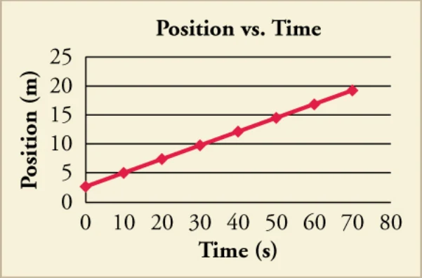
16Calculate the average velocity of the object shown in the graph below over the whole time interval.
16下のグラフに示された物体について、全時間区間にわたる平均速度を計算せよ。
a. 0.25 m/sb. 0.31 m/sc. 3.2 m/sd. 4.00 m/s
a. 0.25 m/sb. 0.31 m/sc. 3.2 m/sd. 4.00 m/s
17True or False: By taking the slope of the curve in the graph you can verify that the velocity of the jet car is at .
17正誤問題:グラフの曲線の傾きをとることで、ジェット車の速度がにおいてであることを確かめられる。
a. Trueb. False
a. 正b. 誤
Check Your Understanding理解の確認
18Which of the following information about motion can be determined by looking at a position vs. time graph that is a straight line?
18直線になっている位置–時間グラフを見ることで分かる運動の情報は、次のうちどれか。
a. frame of referenceb. average acceleration
a. 基準系b. 平均加速度
c. velocityd. direction of force applied
c. 速度d. 加えられた力の向き
19True or False: The position vs time graph of an object that is speeding up is a straight line.a. Trueb. False
19正誤問題:速さを増している物体の位置–時間グラフは直線である。a. 正b. 誤