第2章一次元の運動Motion in One Dimension原書 p.55–96

2.4 Velocity vs. Time Graphs2.4 速度–時間グラフ

SECTION LEARNING OBJECTIVES By the end of this section, you will be able to do the following:

この節の学習目標 この節を終えると、次のことができるようになる。

• Explain the meaning of slope and area in velocity vs. time graphs• Solve problems using velocity vs. time graphs

・速度–時間グラフにおける傾きと面積の意味を説明する・速度–時間グラフを使って問題を解く

Section Key Termsこの節の重要語

acceleration

加速度

Graphing Velocity as a Function of Time速度を時間の関数としてグラフに描く

Earlier, we examined graphs of position versus time. Now, we are going to build on that information as we look at graphs of velocity vs. time. Velocity is the rate of change of displacement. Acceleration is the rate of change of velocity; we will discuss acceleration more in another chapter. These concepts are all very interrelated.

先に位置–時間グラフを調べた。今度はそれを踏まえて、速度–時間グラフを見ていく。速度は変位の変化する割合である。加速度は速度の変化する割合であり、加速度については別の章でさらに論じる。これらの概念はすべて互いに深く結びついている。

VIRTUAL PHYSICSシミュレーションMaze Game迷路ゲーム

In this simulation (https://openstax.org/l/28mazegame) you will use a vector diagram to manipulate a ball into a certain location without hitting a wall. You can manipulate the ball directly with position or by changing its velocity. Explore how these factors change the motion. If you would like, you can put it on the a setting, as well. This is acceleration, which measures the rate of change of velocity. We will explore acceleration in more detail later, but it might be interesting to take a look at it here.

このシミュレーション(https://openstax.org/l/28mazegame)では、ベクトル図を使って、壁にぶつけずにボールを目的の場所へ運ぶ。ボールは位置で直接動かすこともできるし、速度を変えて動かすこともできる。これらがどう運動を変えるか探ってみよう。よければaの設定にしてもよい。これは加速度、すなわち速度の変化する割合である。加速度はあとで詳しく扱うが、ここで少し覗いてみるのも面白いだろう。

If a person takes 3 steps and ends up in the exact same place as their starting point, what must be true?a. The three steps must have equal displacementb. The displacement of the third step is larger than the displacement of the first two.

ある人が3歩進んで、出発点とまったく同じ場所に戻ったとすると、何が成り立っているはずか。a. 3歩の変位は等しいはずである。b. 3歩目の変位は最初の2歩の変位より大きいはずである。

c. The average velocity must add up to zero.d. The distance and average velocity must add up to zero.

c. 平均速度を足し合わせると0になるはずである。d. 道のりと平均速度を足し合わせると0になるはずである。

What can we learn about motion by looking at velocity vs. time graphs? Let’s return to our drive to school, and look at a graph of position versus time as shown in Figure 2.15.

速度–時間グラフを見ることで、運動について何が学べるか。学校への運転に戻って、図2.15の位置–時間グラフを見てみよう。

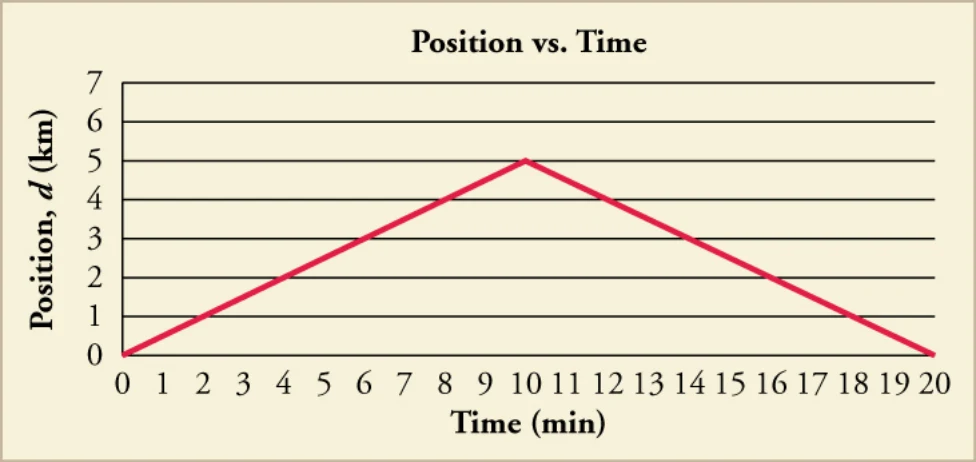
FIGURE 2.15 A graph of position versus time for the drive to and from school is shown.図2.15 学校への行きと帰りの運転についての位置–時間グラフ。

We assumed for our original calculation that your parent drove with a constant velocity to and from school. We now know that the car could not have gone from rest to a constant velocity without speeding up. So the actual graph would be curved on either end, but let’s make the same approximation as we did then, anyway.

最初の計算では、親が学校への行きも帰りも一定の速度で運転したと仮定した。しかし今なら、車が静止から一定の速度になるには加速しなければならないと分かる。だから実際のグラフは両端が曲がっているはずだが、ここでもそのときと同じ近似をしておこう。

TIPS FOR SUCCESS It is common in physics, especially at the early learning stages, for certain things to be neglected, as we see here.

学習のポイント 物理では、とくに学び始めの段階では、ここで見たようにあるものを無視することがよくある。

This is because it makes the concept clearer or the calculation easier. Practicing physicists use these kinds of short-cuts, as well. It works out because usually the thing being neglected is small enough that it does not significantly affect the answer. In the earlier example, the amount of time it takes the car to speed up and reach its cruising velocity is very small compared to the total time traveled.

そのほうが概念がはっきりしたり、計算が楽になったりするからである。現役の物理学者もこうした近道を使う。うまくいくのは、たいていの場合、無視されるものが十分に小さくて答えに大きく響かないからである。先の例では、車が加速して巡航速度に達するまでの時間は、移動時間の合計に比べてごく短い。

Looking at this graph, and given what we learned, we can see that there are two distinct periods to the car’s motion—the way to school and the way back. The average velocity for the drive to school is 0.5 km/minute. We can see that the average velocity for the drive back is –0.5 km/minute. If we plot the data showing velocity versus time, we get another graph (Figure 2.16):

このグラフを、これまで学んだことをふまえて見ると、車の運動にははっきり違う二つの期間、すなわち学校への行きと帰りがあることがわかる。学校への行きの平均速度は0.5 km/分である。帰りの平均速度は−0.5 km/分だとわかる。速度と時間のデータを描けば、別のグラフが得られる(図2.16)。

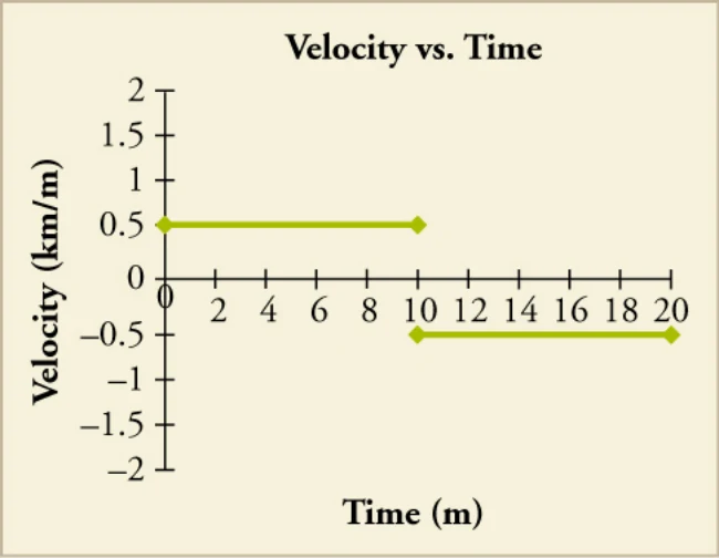
FIGURE 2.16 Graph of velocity versus time for the drive to and from school.図2.16 学校への行きと帰りの運転についての速度–時間グラフ。

We can learn a few things. First, we can derive a v versus t graph from a d versus t graph. Second, if we have a straight-line position–time graph that is positively or negatively sloped, it will yield a horizontal velocity graph. There are a few other interesting things to note. Just as we could use a position vs. time graph to determine velocity, we can use a velocity vs. time graph to determine position. We know that v = d/t. If we use a little algebra to re-arrange the equation, we see that d = v $\times$ t. In Figure 2.16, we have velocity on the y-axis and time along the x-axis. Let’s take just the first half of the motion. We get 0.5 km/minute $\times$ 10 minutes. The units for minutes cancel each other, and we get 5 km, which is the displacement for the trip to school. If we calculate the same for the return trip, we get –5 km. If we add them together, we see that the net displacement for the whole trip is 0 km, which it should be because we started and ended at the same place.

ここからいくつか学べる。第一に、d–tグラフからv–tグラフを導ける。第二に、正または負の傾きを持つ直線の位置–時間グラフからは、水平な速度のグラフが得られる。ほかにも面白い点がいくつかある。位置–時間グラフから速度を求められたのと同じように、速度–時間グラフから位置を求められる。v = d/t であることは分かっている。少し式を変形すれば d = v $\times$ t となる。図2.16ではy軸に速度、x軸に時間をとっている。運動の前半だけをとってみよう。0.5 km/分 $\times$ 10分となる。分の単位が打ち消し合って5 kmが得られ、これが学校までの変位である。帰りについて同じ計算をすると−5 kmが得られる。二つを足せば、全行程の正味の変位は0 kmになる。同じ場所で出発して終わったのだから、そうなるはずである。

TIPS FOR SUCCESS You can treat units just like you treat numbers, so a km/km=1 (or, we say, it cancels out). This is good because it can tell us whether or not we have calculated everything with the correct units. For instance, if we end up with m × s for velocity instead of m/s, we know that something has gone wrong, and we need to check our math. This process is called dimensional analysis, and it is one of the best ways to check if your math makes sense in physics.

学習のポイント 単位は数と同じように扱えるので、km/km = 1 になる(打ち消し合う、という言い方をする)。これは、すべてを正しい単位で計算できたかどうかを教えてくれるので都合がよい。たとえば速度としてm/sではなくm×sが出てきたら、どこかが間違っているとわかるので、計算を見直す必要がある。この手続きを次元解析といい、物理で計算の筋が通っているかを確かめる最良の方法の一つである。

The area under a velocity curve represents the displacement. The velocity curve also tells us whether the car is speeding up. In our earlier example, we stated that the velocity was constant. So, the car is not speeding up.Graphically, you can see that the slope of these two lines is 0. This slope tells us that the car is not speeding up, or accelerating. We will do more with this information in a later chapter. For now, just remember that the area under the graph and the slope are the two important parts of the graph. Just like we could define a linear equation for the motion in a position vs. time graph, we can also define one for a velocity vs. time graph. As we said, the slope equals the acceleration, a. And in this graph, the y-intercept is v₀. Thus, $v = v_{0} + a t$ .

速度の曲線の下の面積は変位を表す。速度の曲線は、車が加速しているかどうかも教えてくれる。先の例では速度は一定だとした。だから車は加速していない。グラフの上では、この2本の直線の傾きが0であることが見て取れる。この傾きは、車が加速していないことを教えてくれる。この情報については後の章でさらに扱う。今は、グラフの下の面積と傾きがグラフの重要な二つの部分だ、とだけ覚えておこう。位置–時間グラフの運動について一次式を定められたのと同じように、速度–時間グラフについても一次式を定められる。すでに述べたとおり、傾きは加速度aに等しい。そしてこのグラフではy切片がv₀である。したがって $v = v_{0} + a t$ となる。

But what if the velocity is not constant? Let’s look back at our jet-car example. At the beginning of the motion, as the car is speeding up, we saw that its position is a curve, as shown in Figure 2.17.

では、速度が一定でなければどうなるか。ジェット車の例に戻ろう。運動の初め、車が加速している間、位置は図2.17のような曲線になるのだった。

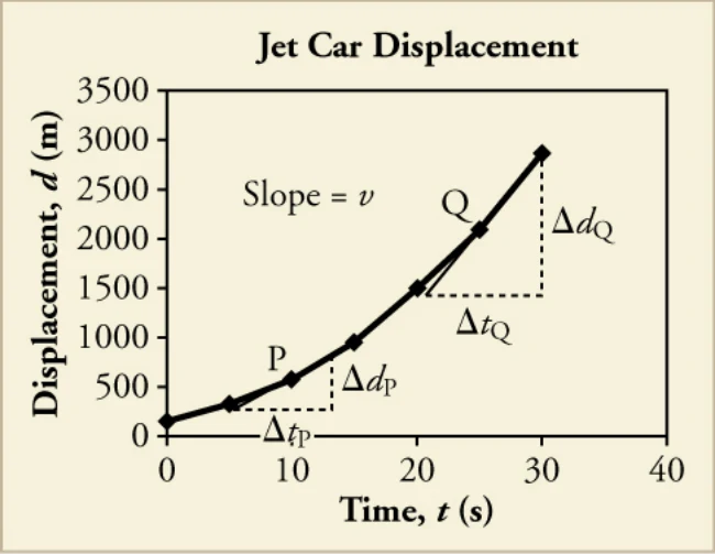
FIGURE 2.17 A graph is shown of the position of a jet-powered car during the time span when it is speeding up. The slope of a d vs. t graph is velocity. This is shown at two points. Instantaneous velocity at any point is the slope of the tangent at that point.図2.17 ジェット推進車が加速している時間帯の位置のグラフ。d–tグラフの傾きは速度である。2点についてそれを示してある。任意の点における瞬間速度は、その点における接線の傾きである。

You do not have to do this, but you could, theoretically, take the instantaneous velocity at each point on this graph. If you did, you would get Figure 2.18, which is just a straight line with a positive slope.

やる必要はないが、理屈のうえでは、このグラフの各点で瞬間速度をとることができる。そうすれば図2.18が得られる。これは正の傾きを持つただの直線である。

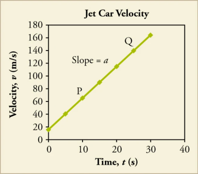
FIGURE 2.18 The graph shows the velocity of a jet-powered car during the time span when it is speeding up.図2.18 ジェット推進車が加速している時間帯の速度のグラフ。

Again, if we take the slope of the velocity vs. time graph, we get the acceleration, the rate of change of the velocity. And, if we take the area under the slope, we get back to the displacement.

ここでも、速度–時間グラフの傾きをとれば加速度、すなわち速度の変化する割合が得られる。そして、速度–時間グラフと時間軸の間の符号付き面積を求めれば、変位が得られる。

Solving Problems using Velocity–Time Graphs速度–時間グラフを使って問題を解く

Most velocity vs. time graphs will be straight lines. When this is the case, our calculations are fairly simple.

たいていの速度–時間グラフは直線になる。その場合、計算はかなり簡単である。

Using Velocity Graph to Calculate Some Stuff: Jet Car Use this figure to (a) find the displacement of the jet car over the time shown (b) calculate the rate of change (acceleration) of the velocity. (c) give the instantaneous velocity at 5 s, and (d) calculate the average velocity over the interval shown.Strategy

速度のグラフを使っていろいろ計算する:ジェット車 この図を使って、(a)示された時間にわたるジェット車の変位を求めよ。(b)速度の変化する割合(加速度)を計算せよ。(c)5 sにおける瞬間速度を答えよ。(d)示された区間の平均速度を計算せよ。方針

a. The displacement is given by finding the area under the line in the velocity vs. time graph.b. The acceleration is given by finding the slope of the velocity graph.

a. 変位は、速度–時間グラフの線の下の面積を求めれば得られる。b. 加速度は、速度のグラフの傾きを求めれば得られる。

c. The instantaneous velocity can just be read off of the graph.

c. 瞬間速度はグラフからそのまま読み取ればよい。

d. To find the average velocity, recall that

d. 平均速度を求めるには、次の式を思い出す。

Solution解答

a.1. Analyze the shape of the area to be calculated. In this case, the area is made up of a rectangle between 0 and 20 m/s stretching to 30 s. The area of a rectangle is length $\times$ width. Therefore, the area of this piece is 600 m.2. Above that is a triangle whose base is 30 s and height is 140 m/s. The area of a triangle is 0.5 $\times$ length $\times$ width. The area of this piece, therefore, is 2,100 m.3. Add them together to get a net displacement of 2,700 m.b. 1. Take two points on the velocity line. Say, t = 5 s and t = 25 s. At t = 5 s, the value of v = 40 m/s. At t = 25 s, v = 140 m/s.

a.1. 求めたい面積の形を調べる。この場合、面積は0から20 m/sの間で30 sまで伸びる長方形と、その上の三角形からなる。長方形の面積は縦 $\times$ 横なので、この部分の面積は600 mである。2. その上は、底辺30 s、高さ140 m/sの三角形である。三角形の面積は0.5 $\times$ 底辺 $\times$ 高さなので、この部分の面積は2,100 mである。3. 足し合わせると正味の変位2,700 mが得られる。b. 1. 速度の直線上に2点をとる。たとえばt = 5 sとt = 25 sとする。t = 5 sではv = 40 m/s、t = 25 sではv = 140 m/sである。

2.Find the slope.

\begin{matrix} a & = & \frac{Δ v}{Δ t} \\ = & \frac{100 m/s}{20 s} \\ = & 5 {m/s}^{2} \end{matrix}

c. The instantaneous velocity at t = 5 s, as we found in part (b) is just 40 m/s.d.1. Find the net displacement, which we found in part (a) was 2,700 m.2. Find the total time which for this case is 30 s.3. Divide 2,700 m/30 s = 90 m/s. Discussion

c. t = 5 sにおける瞬間速度は、(b)で求めたとおり40 m/sである。d.1. 正味の変位を求める。(a)で求めたとおり2,700 mである。2. 全時間を求める。この場合は30 sである。3. 2,700 m ÷ 30 s = 90 m/s。考察

The average velocity we calculated here makes sense if we look at the graph. 100m/s falls about halfway across the graph and since it is a straight line, we would expect about half the velocity to be above and half below.

ここで計算した平均速度は、グラフを見れば納得がいく。100 m/sはグラフのちょうど半ばあたりで、直線なのだから、速度の半分がそれより上、半分が下にあると考えられるからである。

TIPS FOR SUCCESS You can have negative position, velocity, and acceleration on a graph that describes the way the object is moving. You should never see a graph with negative time on an axis. Why?

学習のポイント 物体の動きを表すグラフでは、位置・速度・加速度が負になることはありうる。この章では、観測を始めた時刻を0とし、それ以降の運動を扱う。したがって、グラフには負の時刻は現れない。なぜだろうか。

Most of the velocity vs. time graphs we will look at will be simple to interpret. Occasionally, we will look at curved graphs of velocity vs. time. More often, these curved graphs occur when something is speeding up, often from rest. Let’s look back at a more realistic velocity vs. time graph of the jet car’s motion that takes this speeding up stage into account.

これから見る速度–時間グラフのほとんどは、読み取りが簡単なものである。ときには曲線の速度–時間グラフを見ることもある。そうした曲線のグラフは、たいてい何かが、しばしば静止から、速さを増しているときに現れる。この加速の段階まで考えに入れた、より現実に近いジェット車の速度–時間グラフに戻ってみよう。

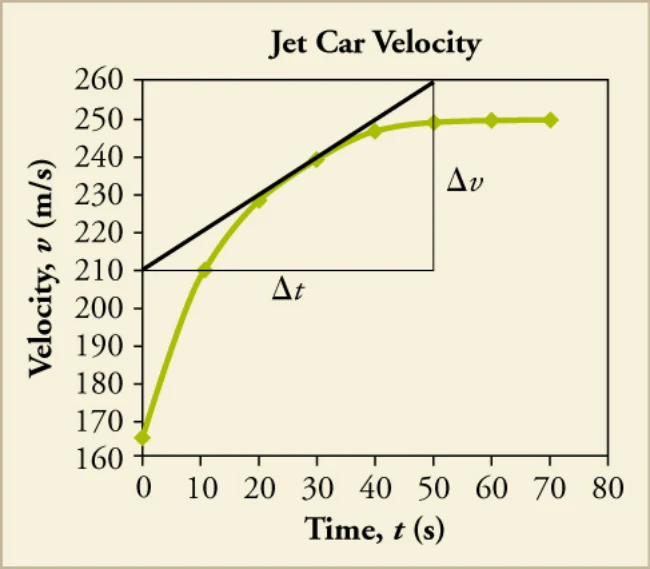
FIGURE 2.19 The graph shows a more accurate graph of the velocity of a jet-powered car during the time span when it is speeding up.図2.19 ジェット推進車が加速している時間帯の速度を、より正確に描いたグラフ。

Using Curvy Velocity Graph to Calculate Some Stuff: Jet Car, Take Two Use Figure 2.19 to (a) find the approximate displacement of the jet car over the time shown, (b) calculate the instantaneous acceleration at t = 30 s, (c) find the instantaneous velocity at 30 s, and (d) calculate the approximate average velocity over the interval shown.Strategy

曲がった速度グラフを使っていろいろ計算する:ジェット車、その2 図2.19を使って、(a)示された時間にわたるジェット車のおよその変位を求めよ。(b)t = 30 sにおける瞬間加速度を計算せよ。(c)30 sにおける瞬間速度を求めよ。(d)示された区間のおよその平均速度を計算せよ。方針

a. Because this graph is an undefined curve, we have to estimate shapes over smaller intervals in order to find the areas.b. Like when we were working with a curved displacement graph, we will need to take a tangent line at the instant we are interested and use that to calculate the instantaneous acceleration.c. The instantaneous velocity can still be read off of the graph.d. We will find the average velocity the same way we did in the previous example. Solution

a. このグラフでは曲線を表す式が与えられていないので、面積を求めるには短い区間ごとに形を見積もらねばならない。b. 曲がった変位のグラフを扱ったときと同じく、関心のある瞬間に接線を引き、それを使って瞬間加速度を計算する必要がある。c. 瞬間速度はやはりグラフから読み取れる。d. 平均速度は前の例と同じやり方で求める。解答

a.1. This problem is more complicated than the last example. To get a good estimate, we should probably break the curve into four sections. 0 → 10 s, 10 → 20 s, 20 → 40 s, and 40 → 70 s.2. Calculate the bottom rectangle (common to all pieces). 165 m/s $\times$ 70 s = 11,550 m.3. Estimate a triangle at the top, and calculate the area for each section. Section 1 contributes a triangle of width 10 s and height (210 – 165) m/s = 45 m/s so the added areas for Section 1 = (1/2)(45 m/s)(10 s) = 225 m; section 2 contributes a rectangle and a triangle with area = 100 m + 450 m = 550 m; section 3 = 150 m + 1,300 m = 1,450 m; section 4 = 2,550 m.4. Add them together to get a net displacement of 16,325 m.b. Using the tangent line given, we find that the slope is 1 m/s².

a.1. この問題は前の例より込み入っている。よい見積もりを得るには、曲線を四つの区間に分けるのがよいだろう。0→10 s、10→20 s、20→40 s、40→70 sである。2. 下側の長方形(全区間に共通)を計算する。165 m/s $\times$ 70 s = 11,550 m。3. 上側を三角形とみなし、各区間の面積を計算する。区間1は幅10 s、高さ(210 − 165) m/s = 45 m/sの三角形なので、区間1の加算面積は(1/2)(45 m/s)(10 s) = 225 m。区間2は長方形と三角形からなり、面積は100 m + 450 m = 550 m。区間3は150 m + 1,300 m = 1,450 m。区間4は2,550 m。4. 足し合わせると正味の変位16,325 mが得られる。b. 与えられた接線を使うと、傾きは1 m/s²と求まる。

c. The instantaneous velocity at t = 30 s, is 240 m/s.d.1. Find the net displacement, which we found in part (a), was 16,325 m.2. Find the total time, which for this case is 70 s.

c. t = 30 sにおける瞬間速度は240 m/sである。d.1. 正味の変位を求める。(a)で求めたとおり16,325 mである。2. 全時間を求める。この場合は70 sである。

3. Divide Discussion3. 割り算する考察

Divide

\frac{16,325 m}{70 s} \sim 233 m/s

This is a much more complicated process than the first problem. If we were to use these estimates to come up with the average velocity over just the first 30 s we would get about 191 m/s. By approximating that curve with a line, we get an average velocity of 202.5 m/s. Depending on our purposes and how precise an answer we need, sometimes calling a curve a straight line is a worthwhile approximation.

これは最初の問題よりずっと込み入った手続きである。この見積もりを使って最初の30秒間だけの平均速度を出すと、およそ191 m/sになる。あの曲線を直線で近似すると、平均速度は202.5 m/sになる。目的と、どれくらい精密な答えが要るかによっては、曲線を直線と呼んでしまうのは値打ちのある近似である。

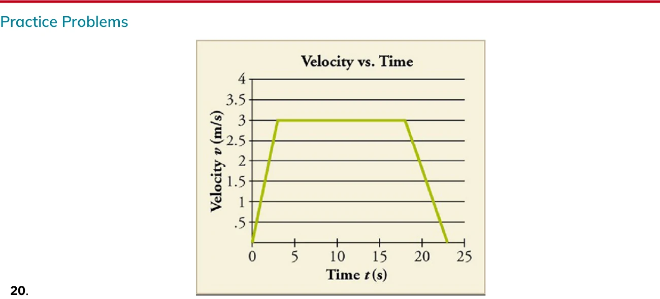
Consider the velocity vs. time graph shown below of a person in an elevator. Suppose the elevator is initially at rest. It then speeds up for 3 seconds, maintains that velocity for 15 seconds, then slows down for 5 seconds until it stops. Find the instantaneous velocity at t = 10 s and t = 23 s.

下に示したのは、エレベーターに乗っている人の速度–時間グラフである。エレベーターは初め静止しているとする。それから3秒間加速し、その速度を15秒間保ち、次の5秒間で減速して止まる。t = 10 sとt = 23 sにおける瞬間速度を求めよ。

a. Instantaneous velocity at t = 10 s and t = 23 s are 0 m/s and 0 m/s.b. Instantaneous velocity at t = 10 s and t = 23 s are 0 m/s and 3 m/s.

a. t = 10 sとt = 23 sにおける瞬間速度は0 m/sと0 m/s。b. t = 10 sとt = 23 sにおける瞬間速度は0 m/sと3 m/s。

c. Instantaneous velocity at t = 10 s and t = 23 s are 3 m/s and 0 m/s.d. Instantaneous velocity at t = 10 s and t = 23 s are 3 m/s and 1.5 m/s.

c. t = 10 sとt = 23 sにおける瞬間速度は3 m/sと0 m/s。d. t = 10 sとt = 23 sにおける瞬間速度は3 m/sと1.5 m/s。

21 .

21.

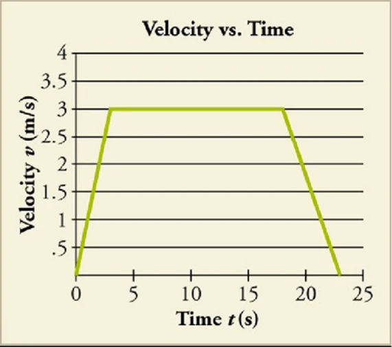
Calculate the net displacement and the average velocity of the elevator over the time interval shown.a. Net displacement is 45 m and average velocity is 2.10 m/s.b. Net displacement is 45 m and average velocity is 2.28 m/s.

示された時間区間について、エレベーターの正味の変位と平均速度を計算せよ。a. 正味の変位は45 m、平均速度は2.10 m/s。b. 正味の変位は45 m、平均速度は2.28 m/s。

c. Net displacement is 57 m and average velocity is 2.66 m/s.d. Net displacement is 57 m and average velocity is 2.48 m/s.

c. 正味の変位は57 m、平均速度は2.66 m/s。d. 正味の変位は57 m、平均速度は2.48 m/s。

SNAP LAB身近な実験Graphing Motion, Take Two運動をグラフにする、その2

In this activity, you will graph a moving ball’s velocity vs. time.

この活動では、動くボールの速度–時間グラフを描く。

• your graph from the earlier Graphing Motion Snap Lab!• 1 piece of graph paper• 1 pencil

・先の「運動をグラフにする」身近な実験で描いたグラフ・方眼紙1枚・鉛筆1本

Procedure手順

1. Take your graph from the earlier Graphing Motion Snap Lab! and use it to create a graph of velocity vs. time.2. Use your graph to calculate the displacement.

1. 先の「運動をグラフにする」身近な実験のグラフを使って、速度–時間グラフを作る。2. そのグラフを使って変位を計算する。

22. Describe the graph and explain what it means in terms of velocity and acceleration.a. The graph shows a horizontal line indicating that the ball moved with a constant velocity, that is, it was not accelerating.b. The graph shows a horizontal line indicating that the ball moved with a constant velocity, that is, it was accelerating.c. The graph shows a horizontal line indicating that the ball moved with a variable velocity, that is, it was not accelerating.d. The graph shows a horizontal line indicating that the ball moved with a variable velocity, that is, it was accelerating.

22. このグラフを説明し、速度と加速度の観点から何を意味しているかを述べよ。a. グラフは水平な直線を示しており、ボールが一定の速度で動いたこと、すなわち加速していなかったことを表す。b. グラフは水平な直線を示しており、ボールが一定の速度で動いたこと、すなわち加速していたことを表す。c. グラフは水平な直線を示しており、ボールの速度が変わっていたこと、すなわち加速していなかったことを表す。d. グラフは水平な直線を示しており、ボールの速度が変わっていたこと、すなわち加速していたことを表す。

Check Your Understanding理解の確認

23What information could you obtain by looking at a velocity vs. time graph?a. accelerationb. direction of motion

23速度–時間グラフを見ることで、どんな情報が得られるか。a. 加速度b. 運動の向き

c. reference frame of the motiond. shortest path

c. 運動の基準系d. 最短の道筋

24How would you use a position vs. time graph to construct a velocity vs. time graph and vice versa?a. The slope of a position vs. time curve is used to construct a velocity vs. time curve, and the slope of a velocity vs. time curve is used to construct a position vs. time curve.b. The slope of a position vs. time curve is used to construct a velocity vs. time curve, and the area of a velocity vs. time curve is used to construct a position vs. time curve.c. The area of a position vs. time curve is used to construct a velocity vs. time curve, and the slope of a velocity vs. time curve is used to construct a position vs. time curve.d. The area of a position vs. time curve is used to construct a velocity vs. time curve, and the area of a velocity vs. time curve is used to construct a position vs. time curve.

24位置–時間グラフから速度–時間グラフを、またその逆をどう作るか。a. 位置–時間曲線の傾きから速度–時間曲線を作り、速度–時間曲線の傾きから位置–時間曲線を作る。b. 位置–時間曲線の傾きから速度–時間曲線を作り、速度–時間曲線の面積から位置–時間曲線を作る。c. 位置–時間曲線の面積から速度–時間曲線を作り、速度–時間曲線の傾きから位置–時間曲線を作る。d. 位置–時間曲線の面積から速度–時間曲線を作り、速度–時間曲線の面積から位置–時間曲線を作る。