第1章物理学とは何かWhat is Physics?原書 p.5–54
Graphing in Physics物理におけるグラフ
Most results in science are presented in scientific journal articles using graphs. Graphs present data in a way that is easy to visualize for humans in general, especially someone unfamiliar with what is being studied. They are also useful for presenting large amounts of data or data with complicated trends in an easily-readable way.
科学の成果のほとんどは、学術論文の中でグラフを使って示される。グラフはデータを、人間一般にとって、とりわけ研究対象をよく知らない人にとって、思い描きやすい形で示してくれる。大量のデータや、込み入った傾向をもつデータを、読み取りやすい形で示すのにも役立つ。
One commonly-used graph in physics and other sciences is the line graph, probably because it is the best graph for showing how one quantity changes in response to the other. Let’s build a line graph based on the data in Table 1.5, which shows the measured distance that a train travels from its station versus time. Our two variables, or things that change along the graph, are time in minutes, and distance from the station, in kilometers. Remember that measured data may not have perfect accuracy.
物理をはじめとする科学でよく使われるグラフの一つが折れ線グラフである。おそらく、ある量が別の量に応じてどう変わるかを示すのに、最も適したグラフだからだろう。表1.5のデータをもとに折れ線グラフを作ってみよう。この表は、列車が駅から進んだ距離を時間に対して測ったものである。グラフに沿って変わるもの、すなわち二つの変数は、分で表した時間と、キロメートルで表した駅からの距離である。測定されたデータが完全に正確とは限らないことを忘れずに。
1. Draw the two axes. The horizontal axis, or x-axis, shows the independent variable, which is the variable that is controlled or manipulated. The vertical axis, or y-axis, shows the dependent variable, the non-manipulated variable that changes with (or is dependent on) the value of the independent variable. In the data above, time is the independent variable and should be plotted on the x-axis. Distance from the station is the dependent variable and should be plotted on the y-axis.2. Label each axes on the graph with the name of each variable, followed by the symbol for its units in parentheses. Be sure to leave room so that you can number each axis. In this example, use Time (min) as the label for the x-axis.3. Next, you must determine the best scale to use for numbering each axis. Because the time values on the x-axis are taken every 10 minutes, we could easily number the x-axis from 0 to 70 minutes with a tick mark every 10 minutes. Likewise, the y-axis scale should start low enough and continue high enough to include all of the distance from station values. A scale from 0 km to 160 km should suffice, perhaps with a tick mark every 10 km.
1. 二本の軸を描く。横軸すなわちx軸には独立変数、つまりこちらが制御し操作する変数をとる。縦軸すなわちy軸には従属変数、つまり操作されず、独立変数の値に応じて変わる(独立変数に依存する)変数をとる。上のデータでは時間が独立変数なので、x軸にとるべきである。駅からの距離が従属変数なので、y軸にとるべきである。2. グラフの各軸に、変数の名前と、続けて括弧書きでその単位の記号を書き入れる。各軸に数値を書き込めるよう余白を残しておくこと。この例では、x軸の見出しを「時間(分)」とする。3. 次に、各軸に数値を振るための最適な目盛りを決めねばならない。x軸の時間の値は10分ごとにとられているので、10分ごとに目盛りを刻んで0分から70分まで数値を振ればよい。同様にy軸の目盛りは、駅からの距離の値をすべて含むよう、十分に低いところから始めて十分に高いところまで続ける必要がある。0 kmから160 kmまでの目盛りで足りるだろう。おそらく10 kmごとに目盛りを刻むのがよい。
In general, you want to pick a scale for both axes that 1) shows all of your data, and 2) makes it easy to identify trends in your data. If you make your scale too large, it will be harder to see how your data change. Likewise, the smaller and more fine you make your scale, the more space you will need to make the graph. The number of significant figures in the axis values should be coarser than the number of significant figures in the measurements.
一般に、両方の軸の目盛りは、1)データがすべて入り、2)データの傾向を読み取りやすい、ものを選びたい。目盛りを大きくとりすぎると、データの変化が見えにくくなる。逆に目盛りを細かくするほど、グラフを描くのに広い場所が要る。軸の値の有効数字は、測定値の有効数字より粗くすべきである。
4. Now that your axes are ready, you can begin plotting your data. For the first data point, count along the x-axis until you find the 10 min tick mark. Then, count up from that point to the 10 km tick mark on the y-axis, and approximate where 22 km is along the y-axis. Place a dot at this location. Repeat for the other six data points (Figure 1.26).
4. 軸が用意できたら、データを打点しはじめられる。最初のデータ点なら、x軸に沿って10分の目盛りまで進む。次にその点からy軸の10 kmの目盛りまで上がり、y軸に沿って22 kmがどこかを見当づける。その位置に点を打つ。残り6個のデータ点についても同じことを繰り返す(図1.26)。
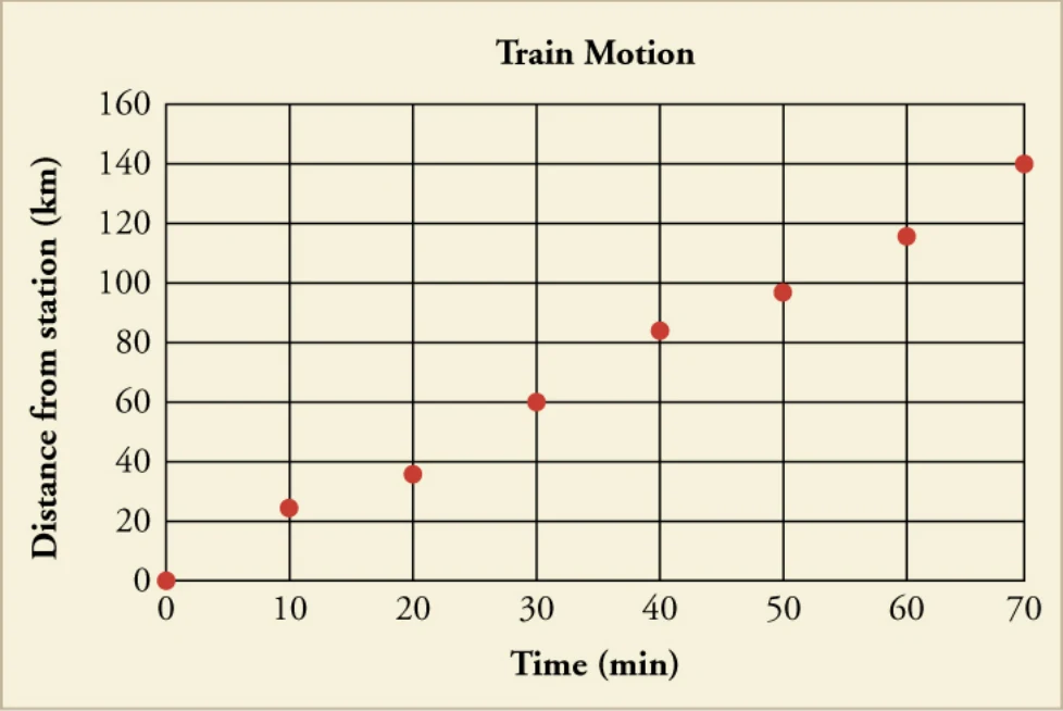
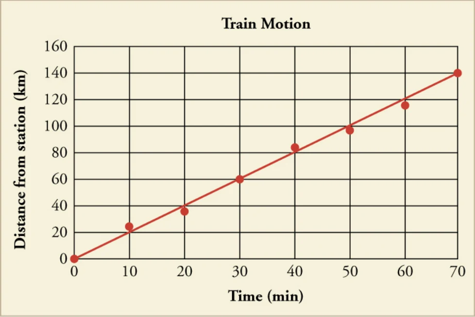
5. Add a title to the top of the graph to state what the graph is describing, such as the y-axis parameter vs. the x-axis parameter. In the graph shown here, the title is train motion. It could also be titled distance of the train from the station vs. time.6. Finally, with data points now on the graph, you should draw a trend line (Figure 1.27). The trend line represents the dependence you think the graph represents, so that the person who looks at your graph can see how close it is to the real data. In the present case, since the data points look like they ought to fall on a straight line, you would draw a straight line as the trend line. Draw it to come closest to all the points. Real data may have some inaccuracies, and the plotted points may not all fall on the trend line. In some cases, none of the data points fall exactly on the trend line.
5. グラフが何を表しているのかを述べる表題を上に付ける。たとえば「y軸の量 対 x軸の量」とする。ここに示したグラフの表題は「列車の運動」である。「駅からの列車の距離 対 時間」としてもよい。6. 最後に、データ点が打たれたので、傾向線を引く(図1.27)。傾向線は、そのグラフが表していると自分が考える依存関係を表すもので、グラフを見る人が、それが実際のデータにどれだけ近いかを見て取れるようにする。今の場合、データ点は直線の上に乗りそうに見えるので、傾向線として直線を引くことになる。すべての点にいちばん近くなるように引く。実際のデータには不正確さがありうるので、打った点がすべて傾向線の上に乗るとは限らない。データ点が一つも傾向線の上に正確に乗らない場合もある。
Analyzing a Graph Using Its Equation One way to get a quick snapshot of a dataset is to look at the equation of its trend line. If the graph produces a straight line, the equation of the trend line takes the form
式を使ってグラフを読み解く データの全体像を手早くつかむ一つの方法は、その傾向線の式を見ることである。グラフが直線になるなら、傾向線の式は次の形をとる。
The b in the equation is the y-intercept while the m in the equation is the slope. The y-intercept tells you at what y value the line intersects the y-axis. In the case of the graph above, the y-intercept occurs at 0, at the very beginning of the graph. The y-intercept, therefore, lets you know immediately where on the y-axis the plot line begins.
式のbはy切片、mは傾きである。y切片は、その直線がy軸と交わるyの値を教えてくれる。上のグラフの場合、y切片はグラフのいちばん始めの0にある。したがってy切片を見れば、グラフの線がy軸のどこから始まるかがすぐにわかる。
The m in the equation is the slope. This value describes how much the line on the graph moves up or down on the y-axis along the line’s length. The slope is found using the following equation
式のmは傾きである。この値は、グラフ上の線がその長さに沿ってy軸方向にどれだけ上がる(下がる)かを表す。傾きは次の式で求める。
In order to solve this equation, you need to pick two points on the line (preferably far apart on the line so the slope you calculate describes the line accurately). The quantities Y2 and Y1 represent the y-values from the two points on the line (not data points) that you picked, while X2 and X1 represent the two x-values of the those points.
この式を解くには、線上の2点を選ぶ必要がある(計算した傾きが線を正しく表すよう、なるべく離れた2点を選ぶのがよい)。Y2とY1は、選んだ線上の2点(データ点ではない)のy座標を、X2とX1はその2点のx座標を表す。
What can the slope value tell you about the graph? The slope of a perfectly horizontal line will equal zero, while the slope of a perfectly vertical line will be undefined because you cannot divide by zero. A positive slope indicates that the line moves up the y-axis as the x-value increases while a negative slope means that the line moves down the y-axis. The more negative or positive the slope is, the steeper the line moves up or down, respectively. The slope of our graph in Figure 1.26 is calculated below based on the two endpoints of the line
傾きの値はグラフについて何を教えてくれるのか。完全に水平な線の傾きは0であり、完全に垂直な線の傾きは、0で割ることができないので定義されない。傾きが正なら、xの値が増えるにつれて線がy軸方向に上がっていくことを示し、傾きが負なら線が下がっていくことを示す。傾きが正または負の方向に大きいほど、線はそれぞれ急に上がる、あるいは急に下がる。図1.26のグラフの傾きを、線の両端の2点にもとづいて以下に計算する。
Because the x axis is time in minutes, we would actually be more likely to use the time t as the independent (x-axis) variable and write the equation as
x軸は分単位の時間なので、実際には時間tを独立変数(x軸)として使い、式を次のように書くほうが自然だろう。
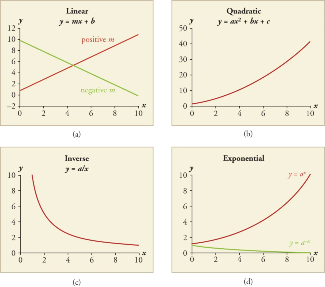
The formula only applies to linear relationships, or ones that produce a straight line. Another common type of line in physics is the quadratic relationship, which occurs when one of the variables is squared. One quadratic relationship in physics is the relation between the speed of an object its centripetal acceleration, which is used to determine the force needed to keep an object moving in a circle. Another common relationship in physics is the inverse relationship, in which one variable decreases whenever the other variable increases. An example in physics is Coulomb’s law. As the distance between two charged objects increases, the electrical force between the two charged objects decreases. Inverse proportionality, such the relation between x and y in the equation
という式は、一次の関係、すなわち直線になる関係にしか当てはまらない。物理でよく出るもう一つの型が二次の関係で、変数の一方が2乗されるときに現れる。物理における二次の関係の一例が、物体の速さとその向心加速度の関係で、これは物体を円運動させ続けるのに必要な力を求めるのに使われる。物理でよく出るもう一つの関係が反比例の関係で、一方の変数が増えるともう一方が減る。物理での例がクーロンの法則である。二つの帯電した物体の距離が増えると、その間にはたらく電気的な力は小さくなる。次の式でxとyの間に表されるような反比例、
for some number k, is one particular kind of inverse relationship. A third commonly-seen relationship is the exponential relationship, in which a change in the independent variable produces a proportional change in the dependent variable. As the value of the dependent variable gets larger, its rate of growth also increases. For example, bacteria often reproduce at an exponential rate when grown under ideal conditions. As each generation passes, there are more and more bacteria to reproduce. As a result, the growth rate of the bacterial population increases every generation (Figure 1.28).
すなわち、xとyが変わってもkが一定に保たれる関係は、反比例の関係の中でも特別な一つの形である。三つ目のよく見る関係が指数関係で、独立変数の変化が従属変数に比例した変化を生むものである。従属変数の値が大きくなるにつれ、その増え方も速くなる。たとえば細菌は、理想的な条件のもとで育てられるとしばしば指数的な速さで増える。世代が進むごとに、増殖する細菌の数がどんどん多くなる。その結果、細菌集団の増加率は世代ごとに大きくなる(図1.28)。
Using Logarithmic Scales in Graphing Sometimes a variable can have a very large range of values. This presents a problem when you’re trying to figure out the best scale to use for your graph’s axes. One option is to use a logarithmic (log) scale. In a logarithmic scale, the value each mark labels is the previous mark’s value multiplied by some constant. For a log base 10 scale, each mark labels a value that is 10 times the value of the mark before it. Therefore, a base 10 logarithmic scale would be numbered: 0, 10, 100, 1,000, etc. You can see how the logarithmic scale covers a much larger range of values than the corresponding linear scale, in which the marks would label the values 0, 10, 20, 30, and so on.
グラフに対数目盛りを使う 変数の値の範囲がとても広いことがある。これは、グラフの軸にどんな目盛りを使うのがよいかを決めるときに困りものである。一つの選択肢が対数目盛りを使うことである。対数目盛りでは、各目盛りが表す値は、一つ前の目盛りの値に一定の数を掛けたものになる。底が10の対数目盛りなら、各目盛りは一つ前の目盛りの10倍の値を表す。したがって底10の対数目盛りには、0、10、100、1,000……と数値が振られる。目盛りが0、10、20、30……となる対応する線形目盛りに比べ、対数目盛りがはるかに広い値の範囲を覆えることがわかるだろう。
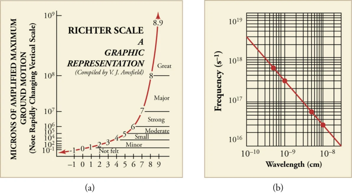
If you use a logarithmic scale on one axis of the graph and a linear scale on the other axis, you are using a semi-log plot. The Richter scale, which measures the strength of earthquakes, uses a semi-log plot. The degree of ground movement is plotted on a logarithmic scale against the assigned intensity level of the earthquake, which ranges linearly from 1-10 (Figure 1.29 (a)).
グラフの一方の軸に対数目盛り、もう一方に線形目盛りを使うと、片対数プロットになる。地震の強さを測るリヒター・スケールは片対数プロットを使っている。地面の動きの大きさを対数目盛りにとり、1から10まで線形に割り振られた地震の強さの階級に対して描く(図1.29(a))。
If a graph has both axes in a logarithmic scale, then it is referred to as a log-log plot. The relationship between the wavelength and frequency of electromagnetic radiation such as light is usually shown as a log-log plot (Figure 1.29 (b)). Log-log plots are also commonly used to describe exponential functions, such as radioactive decay.
グラフの両方の軸が対数目盛りなら、それは両対数プロットと呼ばれる。光のような電磁波の波長と振動数の関係は、ふつう両対数プロットで示される(図1.29(b))。両対数プロットは、放射性崩壊のような指数関数を表すのにもよく使われる。
Method of Adding Percents: Shingling Your Roof A series of shingles are used to protect the roof of a home. Using a measuring tape, you measure one shingle and find its dimensions to be 44 cm by 100 cm. Knowing that your measurements are not perfect, you estimate an uncertainty of ±0.5 cm. Following the method of adding percents, what is the area of the shingle, including uncertainty?Strategy
百分率を足し合わせる方法:屋根を葺く 家の屋根を守るために、屋根板を何枚も使う。巻き尺で1枚を測ったところ、寸法は44 cm×100 cmだった。測定が完全ではないと知っているので、不確かさを±0.5 cmと見積もる。百分率を足し合わせる方法に従うと、不確かさを含めた屋根板の面積はいくらか。方針
While calculating the area of the shingle is straightforward (44 cm x 100 cm = 4400 cm2), determining the percent uncertainty is more challenging. In order to use the method of adding percents, you must first calculate the percent uncertainty of each measurement.
屋根板の面積の計算そのものは単純である(44 cm×100 cm = 4400 cm2)が、百分率の不確かさを求めるほうは少し難しい。百分率を足し合わせる方法を使うには、まず各測定の百分率の不確かさを計算しなければならない。
Solution解答
Length % Uncertainty: ⯑A/A x 100% = 0.5/44 x 100% = 1.1% Width % Uncertainty: ⯑A/A x 100% = 0.5/100 x 100% = 0.5%
長さの百分率の不確かさ:δA/A×100% = 0.5/44×100% = 1.1% 幅の百分率の不確かさ:δA/A×100% = 0.5/100×100% = 0.5%
Adding Percents: 1.1% + 0.5% = 1.6% uncertainty
百分率を足す:1.1% + 0.5% = 1.6%の不確かさ
Area of the Shingle: 4400 cm2 ± 1.6%
屋根板の面積:4400 cm2 ± 1.6%
Note that this uncertainty can also be expressed in metric terms.
この不確かさは、メートル法の量としても表せる。
1.6% x 4400 cm2 = 70.4 cm2
1.6%×4400 cm2 = 70.4 cm2
Area of the Shingle: 4400 ± 70.4 cm2
屋根板の面積:4400 ± 70.4 cm2
Discussion考察
Knowing the percent uncertainty of a shingle can help a contractor determine the number of shingles needed, and therefore the cost, of roofing a new home. Consider how using smaller shingles would affect this uncertainty, and what role this would play in the cost estimation process.
屋根板の百分率の不確かさを知っていれば、施工業者は新築の屋根を葺くのに必要な枚数、したがって費用を見積もれる。もっと小さい屋根板を使ったらこの不確かさはどうなるか、そしてそれが費用の見積もりにどう効いてくるかを考えてみよう。
VIRTUAL PHYSICSシミュレーションGraphing Lines直線のグラフを描く
In this simulation you will examine how changing the slope and y-intercept of an equation changes the appearance of a plotted line. Select slope-intercept form and drag the blue circles along the line to change the line’s characteristics. Then, play the line game and see if you can determine the slope or y-intercept of a given line.
このシミュレーションでは、式の傾きとy切片を変えると、描かれる直線の見え方がどう変わるかを調べる。傾き・切片の形を選び、線上の青い円をドラッグして線の性質を変えてみよう。そのうえで直線当てゲームを遊び、与えられた直線の傾きやy切片を言い当てられるか試してみよう。
Access multimedia content (http://openstax.org/books/physics/pages/1-3-the-language-of-physics-physical-quantities-and-units)
マルチメディア教材はこちら(http://openstax.org/books/physics/pages/1-3-the-language-of-physics-physical-quantities-and-units)
GRASP CHECK How would the following changes affect a line that is neither horizontal nor vertical and has a positive slope?1. increase the slope but keeping the y-intercept constant2. increase the y-intercept but keeping the slope constanta. Increasing the slope will cause the line to rotate clockwise around the y-intercept. Increasing the y-intercept will cause the line to move vertically up on the graph without changing the line’s slope.b. Increasing the slope will cause the line to rotate counter-clockwise around the y-intercept.
理解の確認 水平でも垂直でもなく、傾きが正である直線に、次の変更を加えるとどうなるか。1. y切片を保ったまま傾きを大きくする2. 傾きを保ったままy切片を大きくするa. 傾きを大きくすると、線はy切片を中心に時計回りに回る。y切片を大きくすると、線は傾きを変えずにグラフ上を垂直に上へ動く。b. 傾きを大きくすると、線はy切片を中心に反時計回りに回る。
Increasing the y-intercept will cause the line to move vertically up on the graph without changing the line’s slope.c. Increasing the slope will cause the line to rotate clockwise around the y-intercept. Increasing the y-intercept will cause the line to move horizontally right on the graph without changing the line’s slope.d. Increasing the slope will cause the line to rotate counter-clockwise around the y-intercept.
y切片を大きくすると、線は傾きを変えずにグラフ上を垂直に上へ動く。c. 傾きを大きくすると、線はy切片を中心に時計回りに回る。y切片を大きくすると、線は傾きを変えずにグラフ上を水平に右へ動く。d. 傾きを大きくすると、線はy切片を中心に反時計回りに回る。
Increasing the y-intercept will cause the line to move horizontally right on the graph without changing the line’s slope.
y切片を大きくすると、線は傾きを変えずにグラフ上を水平に右へ動く。
Check Your Understanding理解の確認
12Identify some advantages of metric units.a. Conversion between units is easier in metric units.b. Comparison of physical quantities is easy in metric units.c. Metric units are more modern than English units.d. Metric units are based on powers of 2.
12メートル法単位の利点をいくつか挙げよ。a. メートル法単位では単位どうしの換算がしやすい。b. メートル法単位では物理量の比較がしやすい。c. メートル法単位はヤード・ポンド法単位より近代的である。d. メートル法単位は2の累乗にもとづいている。
13The length of an American football field is , excluding the end zones. How long is the field in meters? Round to the nearest .a. b.
13アメリカン・フットボールの競技場の長さは、エンドゾーンを除いてである。メートルでは何メートルか。の位で四捨五入せよ。a. b.
14The speed limit on some interstate highways is roughly . How many miles per hour is this if is about ?a. 0.1 mi/hb. 27.8 mi/h
14州間高速道路の制限速度はおよそである。だとすると、これは時速何マイルか。a. 0.1 mi/hb. 27.8 mi/h
c. 62 mi/hd. 160 mi/h
c. 62 mi/hd. 160 mi/h
15Briefly describe the target patterns for accuracy and precision and explain the differences between the two.a. Precision states how much repeated measurements generate the same or closely similar results, while accuracy states how close a measurement is to the true value of the measurement.b. Precision states how close a measurement is to the true value of the measurement, while accuracy states how much repeated measurements generate the same or closely similar result.c. Precision and accuracy are the same thing. They state how much repeated measurements generate the same or closely similar results.d. Precision and accuracy are the same thing. They state how close a measurement is to the true value of the measurement.
15正確さと精密さを表す的の図を簡単に説明し、両者の違いを述べよ。a. 精密さは繰り返した測定がどれだけ同じか近い結果を生むかを表し、正確さは測定値が真の値にどれだけ近いかを表す。b. 精密さは測定値が真の値にどれだけ近いかを表し、正確さは繰り返した測定がどれだけ同じか近い結果を生むかを表す。c. 精密さと正確さは同じものである。どちらも、繰り返した測定がどれだけ同じか近い結果を生むかを表す。d. 精密さと正確さは同じものである。どちらも、測定値が真の値にどれだけ近いかを表す。