第6章指数関数と対数関数Exponential and Logarithmic Functions

6.8 Fitting Exponential Models to Data6.8 データへの指数モデルの当てはめ

Learning Objectives 学習目標

In this section, you will:

この節を終えると、次のことができるようになる。

• Build an exponential model from data.• Build a logarithmic model from data.• Build a logistic model from data.

・資料から指数のモデルを組み立てる。・資料から対数のモデルを組み立てる。・資料からロジスティックのモデルを組み立てる。

In previous sections of this chapter, we were either given a function explicitly to graph or evaluate, or we were given a set of points that were guaranteed to lie on the curve. Then we used algebra to find the equation that fit the points exactly. In this section, we use a modeling technique called regression analysis to find a curve that models data collected from real-world observations. With regression analysis, we don’t expect all the points to lie perfectly on the curve. The idea is to find a model that best fits the data. Then we use the model to make predictions about future events.

この章の前の節では、グラフを描いたり値を求めたりする関数がはっきり与えられているか、必ず曲線上にある点の組が与えられているかのどちらかだった。そして代数を使って、その点にぴったり当てはまる式を求めた。この節では、回帰分析と呼ばれるモデル作りの手法を使って、現実の観測から集めた資料のモデルとなる曲線を求める。回帰分析では、すべての点が曲線の上に完全に乗ることは期待しない。狙いは、資料に最もよく当てはまるモデルを求めることである。そしてそのモデルを使って、これから起こることを予測する。

Do not be confused by the word model. In mathematics, we often use the terms function, equation, and model interchangeably, even though they each have their own formal definition. The term model is typically used to indicate that the equation or function approximates a real-world situation.

モデルという語に惑わされないでほしい。数学では、関数・方程式・モデルという語をしばしば同じ意味で使う。それぞれに正式な定義があるにもかかわらずである。モデルという語はふつう、その方程式や関数が現実の状況を近似することを示すのに使われる。

We will concentrate on three types of regression models in this section: exponential, logarithmic, and logistic. Having already worked with each of these functions gives us an advantage. Knowing their formal definitions, the behavior of their graphs, and some of their real-world applications gives us the opportunity to deepen our understanding. As each regression model is presented, key features and definitions of its associated function are included for review. Take a moment to rethink each of these functions, reflect on the work we’ve done so far, and then explore the ways regression is used to model real-world phenomena.

この節では、三つの種類の回帰のモデルに絞る。指数・対数・ロジスティックである。これらの関数をすでに扱ってきたことが強みになる。その正式な定義、グラフの特徴、現実の応用のいくつかを知っていることで、理解を深める機会が得られる。各回帰のモデルを示すときに、それに関わる関数の主だった特徴と定義を振り返りのために入れてある。少し時間をとってこれらの関数を考え直し、ここまでにしてきたことを振り返り、それから回帰が現実の現象のモデル作りにどう使われるかを調べよう。

Building an Exponential Model from Data資料から指数のモデルを組み立てる

As we’ve learned, there are a multitude of situations that can be modeled by exponential functions, such as investment growth, radioactive decay, atmospheric pressure changes, and temperatures of a cooling object. What do these phenomena have in common? For one thing, all the models either increase or decrease as time moves forward. But that’s not the whole story. It’s the way data increase or decrease that helps us determine whether it is best modeled by an exponential equation. Knowing the behavior of exponential functions in general allows us to recognize when to use exponential regression, so let’s review exponential growth and decay.

学んだとおり、投資の増加、放射性崩壊、大気圧の変化、冷めていく物の温度など、指数関数でモデルが作れる状況は数多くある。これらの現象に共通するものは何か。一つには、どのモデルも時間が進むにつれて増えるか減るかのどちらかである。だがそれで全部ではない。指数の式でモデルを作るのが最も良いかどうかを決める手がかりは、資料の増え方・減り方である。指数関数一般のふるまいを知っていれば、いつ指数回帰を使うかが見分けられる。そこで、指数的な増加と減少を振り返ろう。

Recall that exponential functions have the form $y = a b^{x}$ or $y = A_{0} e^{k x} .$ When performing regression analysis, we use the form most commonly used on graphing utilities, $y = a b^{x} .$ Take a moment to reflect on the characteristics we’ve already learned about the exponential function $y = a b^{x}$ (assume $a > 0) :$

指数関数が $y = a b^{x}$ または $y = A_{0} e^{k x}$ の形をとることを思い出そう。回帰分析をするときは、グラフ作成ツールで最もよく使われる形 $y = a b^{x}$ を使う。少し時間をとって、指数関数 $y = a b^{x}$ についてすでに学んだ特徴を振り返ろう( $a > 0) :$ とする)。

• $b$ must be greater than zero and not equal to one.• The initial value of the model is $y = a .$ If $b > 1,$ the function models exponential growth. As $x$ increases, the outputs of the model increase slowly at first, but then increase more and more rapidly, without bound. If $0 < b < 1,$ the function models exponential decay. As $x$ increases, the outputs for the model decrease rapidly at first and then level off to become asymptotic to the x-axis. In other words, the outputs never become equal to or less than zero.

・ $b$ は0より大きく、1に等しくないものでなければならない。・このモデルの初期値は $y = a$ である。 $b > 1$ なら、この関数は指数的な増加のモデルになる。 $x$ が増えると、モデルの出力は初めゆっくり増え、それからどんどん速く、限りなく増える。 $0 < b < 1$ なら、この関数は指数的な減少のモデルになる。 $x$ が増えると、モデルの出力は初め速く減り、それから水平に落ち着いて x軸に漸近する。言い換えれば、出力が0以下になることは決して無い。

As part of the results, your calculator will display a number known as the correlation coefficient, labeled by the variable $r,$ or $r^{2} .$ (You may have to change the calculator’s settings for these to be shown.) The values are an indication of the “goodness of fit” of the regression equation to the data. We more commonly use the value of $r^{2}$ instead of $r,$ but the closer either value is to 1, the better the regression equation approximates the data.

結果の一部として、電卓は相関係数と呼ばれる数を表示する。変数 $r$ または $r^{2}$ で示される。(これを表示するには電卓の設定を変える必要があるかもしれない。)この値は、回帰の式が資料にどれだけよく当てはまるかを示すものである。 $r$ より $r^{2}$ の値を使うほうが多いが、どちらの値も1に近いほど、回帰の式が資料をよく近似している。

Exponential Regression 指数回帰

Exponential regression is used to model situations in which growth begins slowly and then accelerates rapidly without bound, or where decay begins rapidly and then slows down to get closer and closer to zero. We use the command “ExpReg” on a graphing utility to fit an exponential function to a set of data points. This returns an equation of the form, $y = a b^{x}$

指数回帰は、増加が初めゆっくりで、それから限りなく速まる状況や、減少が初め速く、それから緩んで0にどんどん近づく状況のモデルを作るのに使う。グラフ作成ツールで「ExpReg」という命令を使えば、資料の点の組に指数関数を当てはめられる。これは $y = a b^{x}$ の形の式を返す。

Note that:

次に注意せよ。

• $b$ must be non-negative.• when $b > 1,$ we have an exponential growth model.• when $0 < b < 1,$ we have an exponential decay model.

・ $b$ は0以上でなければならない。・ $b > 1$ のとき、指数的な増加のモデルになる。・ $0 < b < 1$ のとき、指数的な減少のモデルになる。

How To 手順

Given a set of data, perform exponential regression using a graphing utility.

資料の組が与えられたとき、グラフ作成ツールを使って指数回帰を行う。

1. Use the STAT then EDIT menu to enter given data. Clear any existing data from the lists. List the input values in the L1 column. List the output values in the L2 column.2. Graph and observe a scatter plot of the data using the STATPLOT feature. Use ZOOM [9] to adjust axes to fit the data. Verify the data follow an exponential pattern.3. Find the equation that models the data. Select “ExpReg” from the STAT then CALC menu. Use the values returned for a and b to record the model, $y = a b^{x} .$ 4. Graph the model in the same window as the scatterplot to verify it is a good fit for the data.

1. STAT から EDIT のメニューを使って、与えられた資料を入れる。リストにすでに入っている資料は消す。入力値を L1 列に並べる。出力値を L2 列に並べる。2. STATPLOT の機能を使って資料の散布図を描き、見る。ZOOM [9] を使って、資料に合うよう座標軸を調える。資料が指数の傾向に従っていることを確かめる。3. 資料のモデルとなる式を求める。STAT から CALC のメニューで「ExpReg」を選ぶ。返された a と b の値を使って、モデル $y = a b^{x}$ を書き留める。4. 散布図と同じ画面にこのモデルのグラフを描き、資料によく当てはまることを確かめる。

Example 1例1

Using Exponential Regression to Fit a Model to Data指数回帰を使って資料にモデルを当てはめる

In 2007, a university study was published investigating the crash risk of alcohol impaired driving. Data from 2,871 crashes were used to measure the association of a person’s blood alcohol level (BAC) with the risk of being in an accident. Table 1 shows results from the study 9. The relative risk is a measure of how many times more likely a person is to crash. So, for example, a person with a BAC of 0.09 is 3.54 times as likely to crash as a person who has not been drinking alcohol.

2007年、酒に酔った運転の衝突の危険を調べた大学の研究が発表された。2,871件の衝突の資料を使って、人の血中アルコール濃度(BAC)と事故に遭う危険の関わりを測った。表1にこの研究の結果を示す。9 相対危険度は、その人が何倍衝突しやすいかを測ったものである。よって、たとえば BAC が0.09の人は、酒を飲んでいない人の3.54倍衝突しやすい。

Source:

Indiana University Center for Studies of Law in Action, 2007

BAC	0	0.01	0.03	0.05	0.07	0.09
Relative Risk of Crashing衝突の相対危険度	1	1.03	1.06	1.38	2.09	3.54
BAC	0.11	0.13	0.15	0.17	0.19	0.21
Relative Risk of Crashing衝突の相対危険度	6.41	12.6	22.1	39.05	65.32	99.78

a. Let $x$ represent the BAC level, and let $y$ represent the corresponding relative risk. Use exponential regression to fit a model to these data.b. After 6 drinks, a person weighing 160 pounds will have a BAC of about $0.16.$ How many times more likely is a person with this weight to crash if they drive after having a 6-pack of beer? Round to the nearest hundredth.

a. $x$ を BAC の値、 $y$ を対応する相対危険度とする。指数回帰を使って、この資料にモデルを当てはめよ。b. 6杯飲んだ後、体重160ポンドの人の BAC はおよそ $0.16.$ になる。この体重の人が缶ビール6本を飲んで運転すると、何倍衝突しやすくなるか。小数第二位まで丸めよ。

Solution 解答

a. Using the STAT then EDIT menu on a graphing utility, list the BAC values in L1 and the relative risk values in L2. Then use the STATPLOT feature to verify that the scatterplot follows the exponential pattern shown in Figure 1: Figure 1 Use the “ExpReg” command from the STAT then CALC menu to obtain the exponential model, $y = 0.58304829 {(2.20720213 E 10)}^{x}$ Converting from scientific notation, we have: $y = 0.58304829 {(22,072,021,300)}^{x}$ Notice that $r^{2} \approx 0.97$ which indicates the model is a good fit to the data. To see this, graph the model in the same window as the scatterplot to verify it is a good fit as shown in Figure 2: Figure 2b. Use the model to estimate the risk associated with a BAC of $0.16.$ Substitute $0.16$ for $x$ in the model and solve for $y .$ $\begin{array}{l} y & = 0.58304829 {(22,072,021,300)}^{x} & Use the regression model found in part (a) . \\ = 0.58304829 {(22,072,021,300)}^{0.16} & Substitute 0 .16 for x . \\ \approx 26 .35 & Round to the nearest hundredth . \end{array}$ If a 160-pound person drives after having 6 drinks, they are about 26.35 times more likely to crash than if driving while sober.

a. グラフ作成ツールで STAT から EDIT のメニューを使い、BAC の値を L1 に、相対危険度の値を L2 に並べる。そして STATPLOT の機能を使って、散布図が図1に示す指数の傾向に従うことを確かめる: 図1。STAT から CALC のメニューで「ExpReg」の命令を使い、指数のモデル $y = 0.58304829 {(2.20720213 E 10)}^{x}$ を得る。科学的記数法から直すと、次が得られる: $y = 0.58304829 {(22,072,021,300)}^{x}$ 。 $r^{2} \approx 0.97$ であり、このモデルが資料によく当てはまることを示していることに注目しよう。これを見るために、散布図と同じ画面にこのモデルのグラフを描き、図2に示すとおりよく当てはまることを確かめる: 図2。b. このモデルを使って、BAC が $0.16.$ のときの危険を見積もる。モデルの $x$ に $0.16$ を代入し、 $y$ について解く。 $\begin{array}{l} y & = 0.58304829 {(22,072,021,300)}^{x} & （a）で得た回帰モデルを使う . \\ = 0.58304829 {(22,072,021,300)}^{0.16} & Substitute 0 .16 for x . \\ \approx 26 .35 & 小数第2位に丸める \end{array}$ 。体重160ポンドの人が6杯飲んで運転すると、しらふで運転するときのおよそ26.35倍衝突しやすい。

Try It #1やってみよう1

Table 2 shows a recent graduate’s credit card balance each month after graduation.

表2は、最近卒業した人の卒業後の毎月のクレジットカードの残高を示している。

Month月	1	2	3	4	5	6	7	8
Debt ($)負債(ドル)	620.00	761.88	899.80	1039.93	1270.63	1589.04	1851.31	2154.92

ⓐUse exponential regression to fit a model to these data.
ⓑIf spending continues at this rate, what will the graduate’s credit card debt be one year after graduating?

ⓐ指数回帰を使って、この資料にモデルを当てはめよ。ⓑこの調子で使い続けると、卒業から1年後のこの人のクレジットカードの負債はいくらになるか。

Q&A 疑問と答え

Is it reasonable to assume that an exponential regression model will represent a situation indefinitely?

指数回帰のモデルが、ある状況をいつまでも表すと考えるのは理にかなっているか。

No. Remember that models are formed by real-world data gathered for regression. It is usually reasonable to make estimates within the interval of original observation (interpolation). However, when a model is used to make predictions, it is important to use reasoning skills to determine whether the model makes sense for inputs far beyond the original observation interval (extrapolation).

いいえ。モデルは、回帰のために集めた現実の資料から作られることを忘れないでほしい。元の観測の区間の内側で見積もる(内挿する)のは、たいてい理にかなっている。だがモデルを使って予測を立てるときは、元の観測の区間からはるかに離れた入力に対してそのモデルが意味を持つかどうかを、筋道を立てて判断することが大切である(外挿)。

Building a Logarithmic Model from Data資料から対数のモデルを組み立てる

Just as with exponential functions, there are many real-world applications for logarithmic functions: intensity of sound, pH levels of solutions, yields of chemical reactions, production of goods, and growth of infants. As with exponential models, data modeled by logarithmic functions are either always increasing or always decreasing as time moves forward. Again, it is the way they increase or decrease that helps us determine whether a logarithmic model is best.

指数関数と同じく、対数関数にも現実の応用が多くある。音の強さ、溶液の pH の値、化学反応の収率、財の生産、乳児の成長などである。指数のモデルと同じく、対数関数でモデル化される資料は、時間が進むにつれてつねに増えるか、つねに減るかのどちらかである。ここでも、対数のモデルが最も良いかどうかを決める手がかりは、その増え方・減り方である。

Recall that logarithmic functions increase or decrease rapidly at first, but then steadily slow as time moves on. By reflecting on the characteristics we’ve already learned about this function, we can better analyze real world situations that reflect this type of growth or decay. When performing logarithmic regression analysis, we use the form of the logarithmic function most commonly used on graphing utilities, $y = a + b \ln (x) .$ For this function

対数関数は初め速く増えるか減るかし、それから時が進むにつれて着実に緩むことを思い出そう。この関数についてすでに学んだ特徴を振り返れば、この種の増加や減少を映す現実の状況をよりよく調べられる。対数回帰の分析をするときは、グラフ作成ツールで最もよく使われる対数関数の形 $y = a + b \ln (x)$ を使う。この関数について、次が成り立つ。

• All input values, $x,$ must be greater than zero.• The point $(1, a)$ is on the graph of the model.• If $b > 0,$ the model is increasing. Growth increases rapidly at first and then steadily slows over time.• If $b < 0,$ the model is decreasing. Decay occurs rapidly at first and then steadily slows over time.

・すべての入力値 $x$ は0より大きくなければならない。・点 $(1, a)$ はこのモデルのグラフ上にある。・ $b > 0$ なら、このモデルは増加する。増加は初め速く、それから時とともに着実に緩む。・ $b < 0$ なら、このモデルは減少する。減少は初め速く起こり、それから時とともに着実に緩む。

Logarithmic Regression 対数回帰

Logarithmic regression is used to model situations where growth or decay accelerates rapidly at first and then slows over time. We use the command “LnReg” on a graphing utility to fit a logarithmic function to a set of data points. This returns an equation of the form,

対数回帰は、増加や減少が初め速く進み、それから時とともに緩む状況のモデルを作るのに使う。グラフ作成ツールで「LnReg」という命令を使えば、資料の点の組に対数関数を当てはめられる。これは次の形の式を返す。

y = a + b \ln (x)

Note that

次に注意せよ。

• all input values, $x,$ must be non-negative.• when $b > 0,$ the model is increasing.• when $b < 0,$ the model is decreasing.

・すべての入力値 $x$ は0以上でなければならない。・ $b > 0$ のとき、このモデルは増加する。・ $b < 0$ のとき、このモデルは減少する。

How To 手順

Given a set of data, perform logarithmic regression using a graphing utility.

資料の組が与えられたとき、グラフ作成ツールを使って対数回帰を行う。

1. Use the STAT then EDIT menu to enter given data. Clear any existing data from the lists. List the input values in the L1 column. List the output values in the L2 column.2. Graph and observe a scatter plot of the data using the STATPLOT feature. Use ZOOM [9] to adjust axes to fit the data. Verify the data follow a logarithmic pattern.3. Find the equation that models the data. Select “LnReg” from the STAT then CALC menu. Use the values returned for a and b to record the model, $y = a + b \ln (x) .$ 4. Graph the model in the same window as the scatterplot to verify it is a good fit for the data.

1. STAT から EDIT のメニューを使って、与えられた資料を入れる。リストにすでに入っている資料は消す。入力値を L1 列に並べる。出力値を L2 列に並べる。2. STATPLOT の機能を使って資料の散布図を描き、見る。ZOOM [9] を使って、資料に合うよう座標軸を調える。資料が対数の傾向に従っていることを確かめる。3. 資料のモデルとなる式を求める。STAT から CALC のメニューで「LnReg」を選ぶ。返された a と b の値を使って、モデル $y = a + b \ln (x)$ を書き留める。4. 散布図と同じ画面にこのモデルのグラフを描き、資料によく当てはまることを確かめる。

Example 2例2

Using Logarithmic Regression to Fit a Model to Data対数回帰を使って資料にモデルを当てはめる

Due to advances in medicine and higher standards of living, life expectancy has been increasing in most developed countries since the beginning of the 20th century.

医学の進歩と生活水準の向上により、20世紀の初めから、ほとんどの先進国で平均余命が延びている。

Table 3 shows the average life expectancies, in years, of Americans from 1900–201010.

表3に、1900年から2010年までのアメリカ人の平均余命(年)を示す。10

Source:

Center for Disease Control and Prevention, 2013

Year年	1900	1910	1920	1930	1940	1950
Life Expectancy(Years)平均余命(年)	47.3	50.0	54.1	59.7	62.9	68.2
Year年	1960	1970	1980	1990	2000	2010
Life Expectancy(Years)平均余命(年)	69.7	70.8	73.7	75.4	76.8	78.7

ⓐLet $x$ represent time in decades starting with $x = 1$ for the year 1900, $x = 2$ for the year 1910, and so on. Let $y$ represent the corresponding life expectancy. Use logarithmic regression to fit a model to these data.ⓑUse the model to predict the average American life expectancy for the year 2030.

ⓐ $x$ を10年単位の時間とし、1900年を $x = 1$ 、1910年を $x = 2$ 、というように置く。 $y$ を対応する平均余命とする。対数回帰を使って、この資料にモデルを当てはめよ。ⓑこのモデルを使って、2030年のアメリカ人の平均余命を予測せよ。

Solution 解答

ⓐUsing the STAT then EDIT menu on a graphing utility, list the years using values 1–12 in L1 and the corresponding life expectancy in L2. Then use the STATPLOT feature to verify that the scatterplot follows a logarithmic pattern as shown in Figure 3: Figure 3 Use the “LnReg” command from the STAT then CALC menu to obtain the logarithmic model, $y = 42.52722583 + 13.85752327 \ln (x)$ Next, graph the model in the same window as the scatterplot to verify it is a good fit as shown in Figure 4: Figure 4ⓑTo predict the life expectancy of an American in the year 2030, substitute $x = 14$ for the in the model and solve for $y :$ $\begin{array}{l} y & = 42.52722583 + 13.85752327 \ln (x) & Use the regression model found in part (a) . \\ = 42.52722583 + 13.85752327 \ln (14) & Substitute 14 for x . \\ \approx 79 .1 & Round to the nearest tenth. \end{array}$ If life expectancy continues to increase at this pace, the average life expectancy of an American will be 79.1 by the year 2030.

ⓐグラフ作成ツールで STAT から EDIT のメニューを使い、年を1〜12の値として L1 に、対応する平均余命を L2 に並べる。そして STATPLOT の機能を使って、散布図が図3に示すとおり対数の傾向に従うことを確かめる: 図3。STAT から CALC のメニューで「LnReg」の命令を使い、対数のモデル $y = 42.52722583 + 13.85752327 \ln (x)$ を得る。次に、散布図と同じ画面にこのモデルのグラフを描き、図4に示すとおりよく当てはまることを確かめる: 図4。ⓑ2030年のアメリカ人の平均余命を予測するには、モデルに $x = 14$ を代入して $y :$ について解く。 $\begin{array}{l} y & = 42.52722583 + 13.85752327 \ln (x) & （a）で得た回帰モデルを使う . \\ = 42.52722583 + 13.85752327 \ln (14) & Substitute 14 for x . \\ \approx 79 .1 & 小数第1位に丸める。 \end{array}$ 。平均余命がこの調子で延び続けるなら、2030年までにアメリカ人の平均余命は79.1になる。

Try It #2やってみよう2

Sales of a video game released in the year 2000 took off at first, but then steadily slowed as time moved on. Table 4 shows the number of games sold, in thousands, from the years 2000–2010.

2000年に売り出されたあるテレビゲームの売上は初め伸びたが、時が進むにつれて着実に緩んだ。表4に、2000年から2010年までの販売本数(千本)を示す。

Year年	2000	2001	2002	2003	2004	2005
Number Sold (thousands)販売本数(千本)	142	149	154	155	159	161
Year年	2006	2007	2008	2009	2010	-
Number Sold (thousands)販売本数(千本)	163	164	164	166	167	-

ⓐLet $x$ represent time in years starting with $x = 1$ for the year 2000. Let $y$ represent the number of games sold in thousands. Use logarithmic regression to fit a model to these data.ⓑIf games continue to sell at this rate, how many games will sell in 2015? Round to the nearest thousand.

ⓐ $x$ を年単位の時間とし、2000年を $x = 1$ と置く。 $y$ を千本単位の販売本数とする。対数回帰を使って、この資料にモデルを当てはめよ。ⓑこの調子で売れ続けるなら、2015年には何本売れるか。千本単位に丸めよ。

Building a Logistic Model from Data資料からロジスティックのモデルを組み立てる

Like exponential and logarithmic growth, logistic growth increases over time. One of the most notable differences with logistic growth models is that, at a certain point, growth steadily slows and the function approaches an upper bound, or limiting value. Because of this, logistic regression is best for modeling phenomena where there are limits in expansion, such as availability of living space or nutrients.

指数や対数の増加と同じく、ロジスティック増加も時間とともに増える。ロジスティック増加のモデルの最も際立った違いの一つは、ある点で増加が着実に緩み、関数が上限すなわち限りの値に近づくことである。このため、ロジスティック回帰は、住む場所や栄養の入手のように広がりに限りがある現象のモデルを作るのに最も向いている。

It is worth pointing out that logistic functions actually model resource-limited exponential growth. There are many examples of this type of growth in real-world situations, including population growth and spread of disease, rumors, and even stains in fabric. When performing logistic regression analysis, we use the form most commonly used on graphing utilities:

ロジスティック関数が、実は資源に限りのある指数的な増加のモデルであることは指摘しておく価値がある。この種の増加は現実の状況に多くの例がある。個体数の増加、病気や噂の広がり、布の染みの広がりさえそうである。ロジスティック回帰の分析をするときは、グラフ作成ツールで最もよく使われる形を使う。

y = \frac{c}{1 + a e^{- b x}}

Recall that:

次を思い出そう。

• $\frac{c}{1 + a}$ is the initial value of the model.• when $b > 0,$ the model increases rapidly at first until it reaches its point of maximum growth rate, $(\frac{\ln (a)}{b}, \frac{c}{2}) .$ At that point, growth steadily slows and the function becomes asymptotic to the upper bound $y = c .$ • $c$ is the limiting value, sometimes called the carrying capacity, of the model.

・ $\frac{c}{1 + a}$ はこのモデルの初期値である。・ $b > 0$ のとき、このモデルは初め速く増え、増加の割合が最大になる点 $(\frac{\ln (a)}{b}, \frac{c}{2})$ に達する。その点から増加は着実に緩み、この関数は上限 $y = c$ に漸近する。・ $c$ はこのモデルの限りの値で、環境収容力とも呼ばれる。

Logistic Regression ロジスティック回帰

Logistic regression is used to model situations where growth accelerates rapidly at first and then steadily slows to an upper limit. We use the command “Logistic” on a graphing utility to fit a logistic function to a set of data points. This returns an equation of the form

ロジスティック回帰は、増加が初め速く進み、それから着実に緩んで上限に近づく状況のモデルを作るのに使う。グラフ作成ツールで「Logistic」という命令を使えば、資料の点の組にロジスティック関数を当てはめられる。これは次の形の式を返す。

y = \frac{c}{1 + a e^{- b x}}

Note that

次に注意せよ。

• The initial value of the model is $\frac{c}{1 + a} .$ • Output values for the model grow closer and closer to $y = c$ as time increases.

・このモデルの初期値は $\frac{c}{1 + a}$ である。・時間が経つにつれて、このモデルの出力値は $y = c$ にどんどん近づく。

How To 手順

Given a set of data, perform logistic regression using a graphing utility.

資料の組が与えられたとき、グラフ作成ツールを使ってロジスティック回帰を行う。

1. Use the STAT then EDIT menu to enter given data. Clear any existing data from the lists. List the input values in the L1 column. List the output values in the L2 column.2. Graph and observe a scatter plot of the data using the STATPLOT feature. Use ZOOM [9] to adjust axes to fit the data. Verify the data follow a logistic pattern.3. Find the equation that models the data. Select “Logistic” from the STAT then CALC menu. Use the values returned for $a,$ $b,$ and $c$ to record the model, $y = \frac{c}{1 + a e^{- b x}} .$ 4. Graph the model in the same window as the scatterplot to verify it is a good fit for the data.

1. STAT から EDIT のメニューを使って、与えられた資料を入れる。リストにすでに入っている資料は消す。入力値を L1 列に並べる。出力値を L2 列に並べる。2. STATPLOT の機能を使って資料の散布図を描き、見る。ZOOM [9] を使って、資料に合うよう座標軸を調える。資料がロジスティックの傾向に従っていることを確かめる。3. 資料のモデルとなる式を求める。STAT から CALC のメニューで「Logistic」を選ぶ。返された $a$ 、 $b$ 、 $c$ の値を使って、モデル $y = \frac{c}{1 + a e^{- b x}}$ を書き留める。4. 散布図と同じ画面にこのモデルのグラフを描き、資料によく当てはまることを確かめる。

Example 3例3

Using Logistic Regression to Fit a Model to Dataロジスティック回帰を使って資料にモデルを当てはめる

Mobile telephone service has increased rapidly in America since the mid 1990s. Today, almost all residents have cellular service. Table 5 shows the percentage of Americans with cellular service between the years 1995 and 2012 11.

携帯電話の契約は、1990年代半ばからアメリカで急速に増えた。今日、住民のほとんどが携帯電話の契約を持っている。表5に、1995年から2012年までの携帯電話の契約を持つアメリカ人の割合を示す。11

Source:

The World Bank, 2013

Year年	Americans with Cellular Service (%)携帯電話の契約を持つアメリカ人(%)	Year年	Americans with Cellular Service (%)携帯電話の契約を持つアメリカ人(%)
1995	12.69	2004	62.852
1996	16.35	2005	68.63
1997	20.29	2006	76.64
1998	25.08	2007	82.47
1999	30.81	2008	85.68
2000	38.75	2009	89.14
2001	45.00	2010	91.86
2002	49.16	2011	95.28
2003	55.15	2012	98.17

ⓐLet $x$ represent time in years starting with $x = 0$ for the year 1995. Let $y$ represent the corresponding percentage of residents with cellular service. Use logistic regression to fit a model to these data.ⓑUse the model to calculate the percentage of Americans with cell service in the year 2013. Round to the nearest tenth of a percent.ⓒDiscuss the value returned for the upper limit, $c .$ What does this tell you about the model? What would the limiting value be if the model were exact?

ⓐ $x$ を年単位の時間とし、1995年を $x = 0$ と置く。 $y$ を、対応する携帯電話の契約を持つ住民の割合とする。ロジスティック回帰を使って、この資料にモデルを当てはめよ。ⓑこのモデルを使って、2013年に携帯電話の契約を持っていたアメリカ人の割合を計算せよ。百分率の小数第一位まで丸めよ。ⓒ上限 $c$ として返された値を論じよ。それはこのモデルについて何を教えているか。このモデルが厳密なら、限りの値はいくらになるはずか。

Solution 解答

ⓐUsing the STAT then EDIT menu on a graphing utility, list the years using values 0–15 in L1 and the corresponding percentage in L2. Then use the STATPLOT feature to verify that the scatterplot follows a logistic pattern as shown in Figure 5: Figure 5 Use the “Logistic” command from the STAT then CALC menu to obtain the logistic model, $y = \frac{105.7379526}{1 + 6.88328979 e^{- 0.2595440013 x}}$ Next, graph the model in the same window as shown in Figure 6 the scatterplot to verify it is a good fit: Figure 6ⓑTo approximate the percentage of Americans with cellular service in the year 2013, substitute $x = 18$ for the in the model and solve for $y :$ $\begin{array}{l} y & = \frac{105.7379526}{1 + 6.88328979 e^{- 0.2595440013 x}} & Use the regression model found in part (a) . \\ = \frac{105.7379526}{1 + 6.88328979 e^{- 0.2595440013 (18)}} & Substitute 18 for x . \\ \approx 99 .3 & Round to the nearest tenth \end{array}$ According to the model, about 99.3% of Americans had cellular service in 2013.ⓒThe model gives a limiting value of about 105. This means that the maximum possible percentage of Americans with cellular service would be 105%, which is impossible. (How could over 100% of a population have cellular service?) If the model were exact, the limiting value would be $c = 100$ and the model’s outputs would get very close to, but never actually reach 100%. After all, there will always be someone out there without cellular service!

ⓐグラフ作成ツールで STAT から EDIT のメニューを使い、年を0〜15の値として L1 に、対応する割合を L2 に並べる。そして STATPLOT の機能を使って、散布図が図5に示すとおりロジスティックの傾向に従うことを確かめる: 図5。STAT から CALC のメニューで「Logistic」の命令を使い、ロジスティックのモデル $y = \frac{105.7379526}{1 + 6.88328979 e^{- 0.2595440013 x}}$ を得る。次に、図6のように散布図と同じ画面にこのモデルのグラフを描き、よく当てはまることを確かめる: 図6。ⓑ2013年に携帯電話の契約を持っていたアメリカ人の割合を近似するには、モデルに $x = 18$ を代入して $y :$ について解く。 $\begin{array}{l} y & = \frac{105.7379526}{1 + 6.88328979 e^{- 0.2595440013 x}} & （a）で得た回帰モデルを使う . \\ = \frac{105.7379526}{1 + 6.88328979 e^{- 0.2595440013 (18)}} & Substitute 18 for x . \\ \approx 99 .3 & 小数第1位に丸める \end{array}$ 。このモデルによれば、2013年にはおよそ99.3%のアメリカ人が携帯電話の契約を持っていた。ⓒこのモデルはおよそ105という限りの値を与える。つまり、携帯電話の契約を持つアメリカ人の割合の最大は105%になるということだが、これはありえない。(人口の100%を超える人が携帯電話の契約を持つなど、どうすればできるのか。)このモデルが厳密なら、限りの値は $c = 100$ になり、モデルの出力は100%にきわめて近づくが、決してそこに達しないはずである。結局のところ、携帯電話の契約を持たない人はつねにどこかにいるのである。

Try It #3やってみよう3

Table 6 shows the population, in thousands, of harbor seals in the Wadden Sea over the years 1997 to 2012.

表6に、1997年から2012年までのワッデン海のゼニガタアザラシの個体数(千頭)を示す。

Year年	Seal Population (Thousands)アザラシの個体数(千頭)	Year年	Seal Population (Thousands)アザラシの個体数(千頭)
1997	3.493	2005	19.590
1998	5.282	2006	21.955
1999	6.357	2007	22.862
2000	9.201	2008	23.869
2001	11.224	2009	24.243
2002	12.964	2010	24.344
2003	16.226	2011	24.919
2004	18.137	2012	25.108

ⓐLet $x$ represent time in years starting with $x = 0$ for the year 1997. Let $y$ represent the number of seals in thousands. Use logistic regression to fit a model to these data.ⓑUse the model to predict the seal population for the year 2020.ⓒTo the nearest whole number, what is the limiting value of this model?

ⓐ $x$ を年単位の時間とし、1997年を $x = 0$ と置く。 $y$ を千頭単位のアザラシの数とする。ロジスティック回帰を使って、この資料にモデルを当てはめよ。ⓑこのモデルを使って、2020年のアザラシの個体数を予測せよ。ⓒこのモデルの限りの値は、整数でいくらか。

Media 教材

Access this online resource for additional instruction and practice with exponential function models.

指数関数のモデルについての説明と練習をさらに求めるなら、次のオンライン教材にあたるとよい。

• Exponential Regression on a Calculator

・電卓での指数回帰

Verbal言葉で答える問題

1. What situations are best modeled by a logistic equation? Give an example, and state a case for why the example is a good fit.

1. ロジスティックの式で最もよくモデル化できるのはどんな状況か。例を一つ挙げ、その例がよく当てはまる理由を述べよ。

2. What is a carrying capacity? What kind of model has a carrying capacity built into its formula? Why does this make sense?

2. 環境収容力とは何か。どんな種類のモデルが、その公式に環境収容力を組み込んでいるか。それが理にかなうのはなぜか。

3. What is regression analysis? Describe the process of performing regression analysis on a graphing utility.

3. 回帰分析とは何か。グラフ作成ツールで回帰分析を行う手順を述べよ。

4. What might a scatterplot of data points look like if it were best described by a logarithmic model?

4. 対数のモデルで最もよく述べられる資料の点の散布図は、どんな見た目になるか。

5. What does the y-intercept on the graph of a logistic equation correspond to for a population modeled by that equation?

5. ロジスティックの式のグラフの y切片は、その式でモデル化される個体数について何に当たるか。

Graphicalグラフの問題

For the following exercises, match the given function of best fit with the appropriate scatterplot in Figure 7 through Figure 11. Answer using the letter beneath the matching graph.

次の各問について、与えられた最もよく当てはまる関数を、図7から図11のふさわしい散布図に対応させよ。対応するグラフの下の記号で答えよ。

6. $y = 10.209 e^{- 0.294 x}$

7. $y = 5.598 - 1.912 \ln (x)$

8. $y = 2.104 {(1.479)}^{x}$

9. $y = 4.607 + 2.733 \ln (x)$

10. $y = \frac{14.005}{1 + 2.79 e^{- 0.812 x}}$

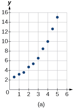
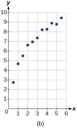
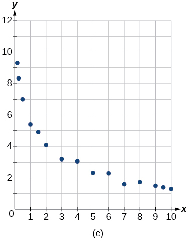
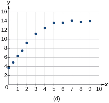
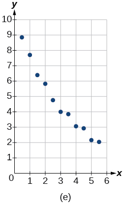
Numeric数値の問題

11. To the nearest whole number, what is the initial value of a population modeled by the logistic equation $P (t) = \frac{175}{1 + 6.995 e^{- 0.68 t}} ?$ What is the carrying capacity?

11. ロジスティックの式 $P (t) = \frac{175}{1 + 6.995 e^{- 0.68 t}} ?$ でモデル化される個体数の初期値は、整数でいくらか。環境収容力はいくらか。

12. Rewrite the exponential model $A (t) = 1550 {(1.085)}^{x}$ as an equivalent model with base $e .$ Express the exponent to four significant digits.

12. 指数のモデル $A (t) = 1550 {(1.085)}^{x}$ を、底 $e$ の同値なモデルに書き直せ。指数は有効数字4桁で表せ。

13. A logarithmic model is given by the equation $h (p) = 67.682 - 5.792 \ln (p) .$ To the nearest hundredth, for what value of $p$ does $h (p) = 62 ?$

13. 対数のモデルが式 $h (p) = 67.682 - 5.792 \ln (p)$ で与えられている。 $h (p) = 62 ?$ となるのは $p$ がいくらのときか。小数第二位まで求めよ。

14. A logistic model is given by the equation $P (t) = \frac{90}{1 + 5 e^{- 0.42 t}} .$ To the nearest hundredth, for what value of t does $P (t) = 45 ?$

14. ロジスティックのモデルが式 $P (t) = \frac{90}{1 + 5 e^{- 0.42 t}}$ で与えられている。 $P (t) = 45 ?$ となるのは t がいくらのときか。小数第二位まで求めよ。

15. What is the y-intercept on the graph of the logistic model given in the previous exercise?

15. 前問で与えられたロジスティックのモデルのグラフの y切片は何か。

Technology機器を使う問題

For the following exercises, use this scenario: The population $P$ of a koi pond over $x$ months is modeled by the function $P (x) = \frac{68}{1 + 16 e^{- 0.28 x}} .$

次の各問では、次の筋書きを使え。 $x$ か月後の錦鯉の池の個体数 $P$ は、関数 $P (x) = \frac{68}{1 + 16 e^{- 0.28 x}}$ でモデル化される。

16. Graph the population model to show the population over a span of $3$ years.

16. $3$ 年にわたる個体数を示すように、この個体数のモデルのグラフを描け。

17. What was the initial population of koi?

17. 錦鯉の初めの数はいくらだったか。

18. How many koi will the pond have after one and a half years?

18. 1年半後、この池には錦鯉が何匹いるか。

19. How many months will it take before there are $20$ koi in the pond?

19. 池の錦鯉が $20$ 匹になるまでに何か月かかるか。

20. Use the intersect feature to approximate the number of months it will take before the population of the pond reaches half its carrying capacity.

20. intersect の機能を使って、池の個体数が環境収容力の半分に達するまでにかかる月数を近似せよ。

For the following exercises, use this scenario: The population $P$ of an endangered species habitat for wolves is modeled by the function $P (x) = \frac{558}{1 + 54.8 e^{- 0.462 x}},$ where $x$ is given in years.

次の各問では、次の筋書きを使え。絶滅危惧種である狼の生息地の個体数 $P$ は、関数 $P (x) = \frac{558}{1 + 54.8 e^{- 0.462 x}}$ でモデル化される。ここで $x$ は年で与えられる。

21. Graph the population model to show the population over a span of $10$ years.

21. $10$ 年にわたる個体数を示すように、この個体数のモデルのグラフを描け。

22. What was the initial population of wolves transported to the habitat?

22. この生息地に移された狼の初めの数はいくらだったか。

23. How many wolves will the habitat have after $3$ years?

23. $3$ 年後、この生息地には狼が何頭いるか。

24. How many years will it take before there are $100$ wolves in the habitat?

24. この生息地の狼が $100$ 頭になるまでに何年かかるか。

25. Use the intersect feature to approximate the number of years it will take before the population of the habitat reaches half its carrying capacity.

25. intersect の機能を使って、この生息地の個体数が環境収容力の半分に達するまでにかかる年数を近似せよ。

For the following exercises, refer to Table 7.

次の各問では、表7を参照せよ。

x	1	2	3	4	5	6
*f(x)*	1125	1495	2310	3294	4650	6361

26. Use a graphing calculator to create a scatter diagram of the data.

26. グラフ電卓を使って、この資料の散布図を作れ。

27. Use the regression feature to find an exponential function that best fits the data in the table.

27. 回帰の機能を使って、表の資料に最もよく当てはまる指数関数を求めよ。

28. Write the exponential function as an exponential equation with base $e .$

28. この指数関数を、底 $e$ の指数の式として書け。

29. Graph the exponential equation on the scatter diagram.

29. この指数の式のグラフを散布図に描け。

30. Use the intersect feature to find the value of $x$ for which $f (x) = 4000.$

30. intersect の機能を使って、 $f (x) = 4000.$ となる $x$ の値を求めよ。

For the following exercises, refer to Table 8.

次の各問では、表8を参照せよ。

x	1	2	3	4	5	6
*f(x)*	555	383	307	210	158	122

31. Use a graphing calculator to create a scatter diagram of the data.

31. グラフ電卓を使って、この資料の散布図を作れ。

32. Use the regression feature to find an exponential function that best fits the data in the table.

32. 回帰の機能を使って、表の資料に最もよく当てはまる指数関数を求めよ。

33. Write the exponential function as an exponential equation with base $e .$

33. この指数関数を、底 $e$ の指数の式として書け。

34. Graph the exponential equation on the scatter diagram.

34. この指数の式のグラフを散布図に描け。

35. Use the intersect feature to find the value of $x$ for which $f (x) = 250.$

35. intersect の機能を使って、 $f (x) = 250.$ となる $x$ の値を求めよ。

For the following exercises, refer to Table 9.

次の各問では、表9を参照せよ。

x	1	2	3	4	5	6
*f(x)*	5.1	6.3	7.3	7.7	8.1	8.6

36. Use a graphing calculator to create a scatter diagram of the data.

36. グラフ電卓を使って、この資料の散布図を作れ。

37. Use the LOGarithm option of the REGression feature to find a logarithmic function of the form $y = a + b \ln (x)$ that best fits the data in the table.

37. 回帰の機能の LOGarithm を使って、表の資料に最もよく当てはまる $y = a + b \ln (x)$ の形の対数関数を求めよ。

38. Use the logarithmic function to find the value of the function when $x = 10.$

38. この対数関数を使って、 $x = 10.$ のときの関数の値を求めよ。

39. Graph the logarithmic equation on the scatter diagram.

39. この対数の式のグラフを散布図に描け。

40. Use the intersect feature to find the value of $x$ for which $f (x) = 7.$

40. intersect の機能を使って、 $f (x) = 7.$ となる $x$ の値を求めよ。

For the following exercises, refer to Table 10.

次の各問では、表10を参照せよ。

x	1	2	3	4	5	6	7	8
*f(x)*	7.5	6	5.2	4.3	3.9	3.4	3.1	2.9

41. Use a graphing calculator to create a scatter diagram of the data.

41. グラフ電卓を使って、この資料の散布図を作れ。

42. Use the LOGarithm option of the REGression feature to find a logarithmic function of the form $y = a + b \ln (x)$ that best fits the data in the table.

42. 回帰の機能の LOGarithm を使って、表の資料に最もよく当てはまる $y = a + b \ln (x)$ の形の対数関数を求めよ。

43. Use the logarithmic function to find the value of the function when $x = 10.$

43. この対数関数を使って、 $x = 10.$ のときの関数の値を求めよ。

44. Graph the logarithmic equation on the scatter diagram.

44. この対数の式のグラフを散布図に描け。

45. Use the intersect feature to find the value of $x$ for which $f (x) = 8.$

45. intersect の機能を使って、 $f (x) = 8.$ となる $x$ の値を求めよ。

For the following exercises, refer to Table 11.

次の各問では、表11を参照せよ。

x	1	2	3	4	5	6	7	8	9	10
*f(x)*	8.7	12.3	15.4	18.5	20.7	22.5	23.3	24	24.6	24.8

46. Use a graphing calculator to create a scatter diagram of the data.

46. グラフ電卓を使って、この資料の散布図を作れ。

47. Use the LOGISTIC regression option to find a logistic growth model of the form $y = \frac{c}{1 + a e^{- b x}}$ that best fits the data in the table.

47. LOGISTIC 回帰を使って、表の資料に最もよく当てはまる $y = \frac{c}{1 + a e^{- b x}}$ の形のロジスティック増加のモデルを求めよ。

48. Graph the logistic equation on the scatter diagram.

48. このロジスティックの式のグラフを散布図に描け。

49. To the nearest whole number, what is the predicted carrying capacity of the model?

49. このモデルが予測する環境収容力は、整数でいくらか。

50. Use the intersect feature to find the value of $x$ for which the model reaches half its carrying capacity.

50. intersect の機能を使って、このモデルが環境収容力の半分に達する $x$ の値を求めよ。

For the following exercises, refer to Table 12.

次の各問では、表12を参照せよ。

$x$	0	2	4	5	7	8	10	11	15	17
$f (x)$	12	28.6	52.8	70.3	99.9	112.5	125.8	127.9	135.1	135.9

51. Use a graphing calculator to create a scatter diagram of the data.

51. グラフ電卓を使って、この資料の散布図を作れ。

52. Use the LOGISTIC regression option to find a logistic growth model of the form $y = \frac{c}{1 + a e^{- b x}}$ that best fits the data in the table.

52. LOGISTIC 回帰を使って、表の資料に最もよく当てはまる $y = \frac{c}{1 + a e^{- b x}}$ の形のロジスティック増加のモデルを求めよ。

53. Graph the logistic equation on the scatter diagram.

53. このロジスティックの式のグラフを散布図に描け。

54. To the nearest whole number, what is the predicted carrying capacity of the model?

54. このモデルが予測する環境収容力は、整数でいくらか。

55. Use the intersect feature to find the value of $x$ for which the model reaches half its carrying capacity.

55. intersect の機能を使って、このモデルが環境収容力の半分に達する $x$ の値を求めよ。

Extensions発展問題

56. Recall that the general form of a logistic equation for a population is given by $P (t) = \frac{c}{1 + a e^{- b t}},$ such that the initial population at time $t = 0$ is $P (0) = P_{0} .$ Show algebraically that $\frac{c - P (t)}{P (t)} = \frac{c - P_{0}}{P_{0}} e^{- b t} .$

56. 個体数のロジスティックの式の一般形が $P (t) = \frac{c}{1 + a e^{- b t}}$ で与えられ、時刻 $t = 0$ の初めの個体数が $P (0) = P_{0}$ であることを思い出そう。 $\frac{c - P (t)}{P (t)} = \frac{c - P_{0}}{P_{0}} e^{- b t}$ を代数的に示せ。

57. Use a graphing utility to find an exponential regression formula $f (x)$ and a logarithmic regression formula $g (x)$ for the points $(1.5, 1.5)$ and $(8.5, 8.5) .$ Round all numbers to 6 decimal places. Graph the points and both formulas along with the line $y = x$ on the same axis. Make a conjecture about the relationship of the regression formulas.

57. グラフ作成ツールを使って、点 $(1.5, 1.5)$ と $(8.5, 8.5)$ について、指数回帰の式 $f (x)$ と対数回帰の式 $g (x)$ を求めよ。すべての数を小数第六位まで丸めよ。これらの点と両方の式を、直線 $y = x$ と一緒に同じ座標軸に描け。この二つの回帰の式の関係について予想を立てよ。

58. Verify the conjecture made in the previous exercise. Round all numbers to six decimal places when necessary.

58. 前問で立てた予想を確かめよ。必要なら、すべての数を小数第六位まで丸めよ。

59. Find the inverse function $f^{- 1} (x)$ for the logistic function $f (x) = \frac{c}{1 + a e^{- b x}} .$ Show all steps.

59. ロジスティック関数 $f (x) = \frac{c}{1 + a e^{- b x}}$ の逆関数 $f^{- 1} (x)$ を求めよ。すべての手順を示せ。

60. Use the result from the previous exercise to graph the logistic model $P (t) = \frac{20}{1 + 4 e^{- 0.5 t}}$ along with its inverse on the same axis. What are the intercepts and asymptotes of each function?

60. 前問の結果を使って、ロジスティックのモデル $P (t) = \frac{20}{1 + 4 e^{- 0.5 t}}$ とその逆関数のグラフを同じ座標軸に描け。それぞれの関数の切片と漸近線は何か。

Key Terms重要語

annual percentage rate (APR) the yearly interest rate earned by an investment account, also called nominal rate

年利(APR) 投資口座が1年に得る利率。名目利率ともいう

carrying capacity in a logistic model, the limiting value of the output

環境収容力 ロジスティックのモデルで、出力の限りの値

change-of-base formula a formula for converting a logarithm with any base to a quotient of logarithms with any other base.

底の変換公式 どんな底の対数も、ほかの任意の底の対数の商に直す公式

common logarithm the exponent to which 10 must be raised to get $x;$ $\log_{10} (x)$ is written simply as $\log (x) .$

常用対数 $x;$ を得るために10を累乗しなければならない指数。 $\log_{10} (x)$ は単に $\log (x)$ と書く

compound interest interest earned on the total balance, not just the principal

複利元金だけでなく、残高の全体につく利子

doubling time the time it takes for a quantity to double

倍加時間 ある量が2倍になるのにかかる時間

exponential growth a model that grows by a rate proportional to the amount present

指数的な増加 現在の量に比例する割合で増えるモデル

extraneous solution a solution introduced while solving an equation that does not satisfy the conditions of the original equation

無縁解 方程式を解く途中で生じる、元の方程式の条件を満たさない解

half-life the length of time it takes for a substance to exponentially decay to half of its original quantity

半減期 ある物質が指数的に減って元の量の半分になるのにかかる時間の長さ

logarithm the exponent to which $b$ must be raised to get $x;$ written $y = \log_{b} (x)$

対数 $x;$ を得るために $b$ を累乗しなければならない指数。 $y = \log_{b} (x)$ と書く

logistic growth model a function of the form $f (x) = \frac{c}{1 + a e^{- b x}}$ where $\frac{c}{1 + a}$ is the initial value, $c$ is the carrying capacity, or limiting value, and $b$ is a constant determined by the rate of growth

ロジスティック増加のモデル $f (x) = \frac{c}{1 + a e^{- b x}}$ の形の関数。 $\frac{c}{1 + a}$ は初期値、 $c$ は環境収容力すなわち限りの値、 $b$ は増加の割合で決まる定数である

natural logarithm the exponent to which the number $e$ must be raised to get $x;$ $\log_{e} (x)$ is written as $\ln (x) .$

自然対数 $x;$ を得るために数 $e$ を累乗しなければならない指数。 $\log_{e} (x)$ は $\ln (x)$ と書く

Newton’s Law of Cooling the scientific formula for temperature as a function of time as an object’s temperature is equalized with the ambient temperature

ニュートンの冷却の法則 物の温度が周りの温度と等しくなっていくときの、時間の関数としての温度を与える科学の公式

nominal rate the yearly interest rate earned by an investment account, also called annual percentage rate

名目利率 投資口座が1年に得る利率。年利ともいう

order of magnitude the power of ten, when a number is expressed in scientific notation, with one non-zero digit to the left of the decimal

桁小数点の左に0でない一桁だけ置いて科学的記数法で表したときの、10の指数

power rule for logarithms a rule of logarithms that states that the log of a power is equal to the product of the exponent and the log of its base

対数の累乗の法則 累乗の対数が、指数と底の対数の積に等しいと述べる対数の法則

product rule for logarithms a rule of logarithms that states that the log of a product is equal to a sum of logarithms

対数の積の法則 積の対数が対数の和に等しいと述べる対数の法則

quotient rule for logarithms a rule of logarithms that states that the log of a quotient is equal to a difference of logarithms

対数の商の法則 商の対数が対数の差に等しいと述べる対数の法則